#!/usr/bin/env python3
"""
===============================================================================
HDGL COUNTER-ROTATING PHYLLOTAXIS — DRAIN EFFECT
===============================================================================

Two simultaneous phyllotactic fields:

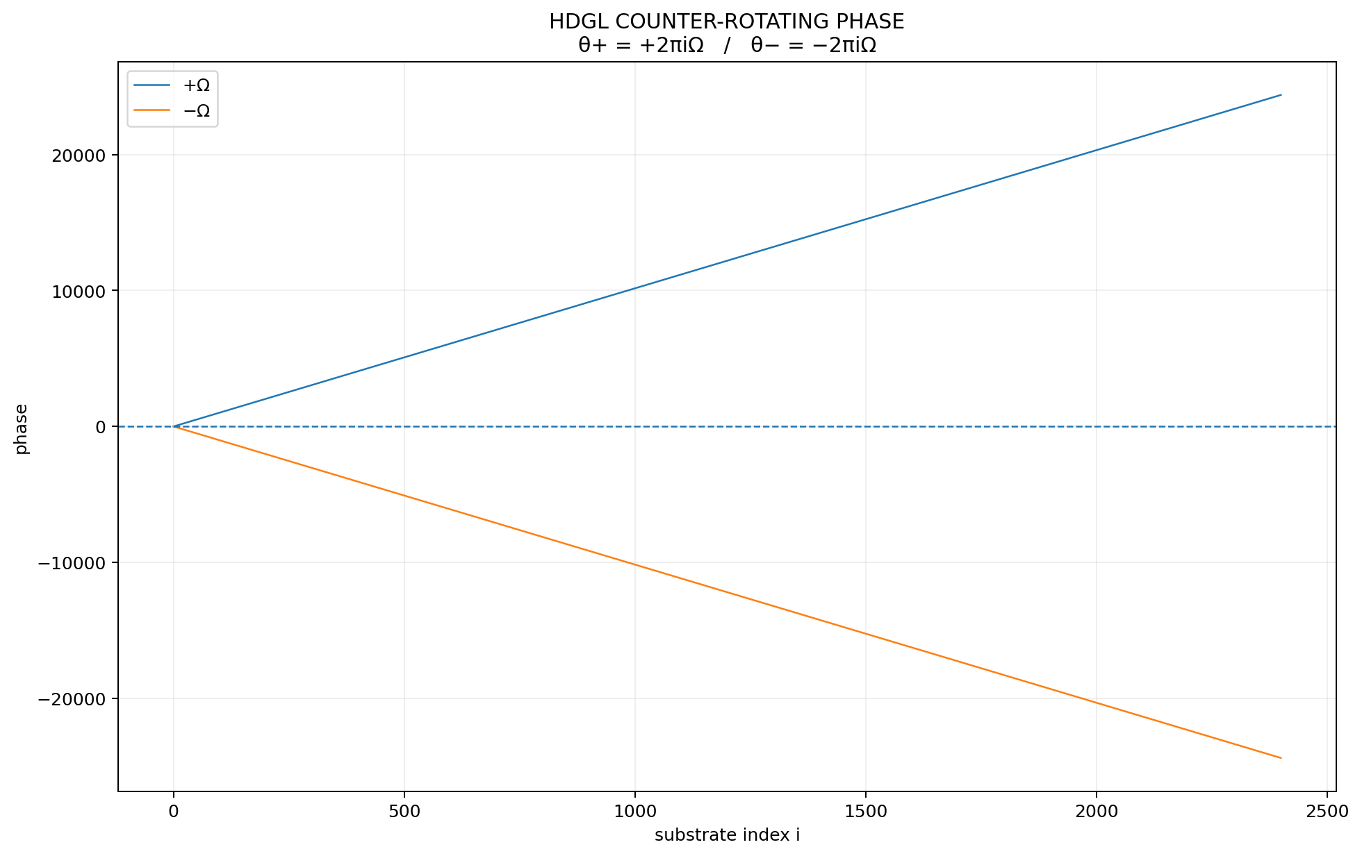
    θ+ = +2π i Ω
    θ- = -2π i Ω

They counter-rotate while sharing one reciprocal radial closure:

    T(X) = 1 + 1/X

The drain is produced by reciprocal compression toward the common origin:

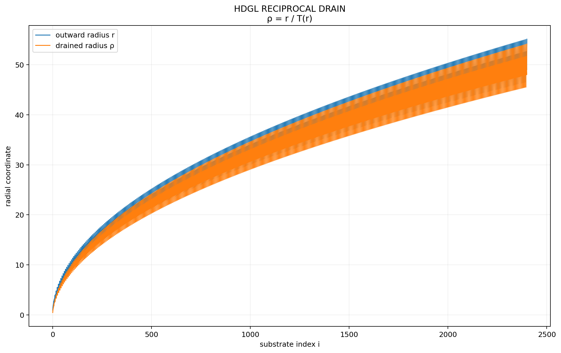
    d(r) = 1 / T(r)

    ρ(r) = r * d(r)

The binary/trinary substrate remains simultaneous:

    B_i ∈ {0,1}
    τ_i ∈ {-1,0,+1}

No stored φ is used.
Ω emerges from:

    Ω_(n+1) = T(Ω_n)
            = 1 + 1/Ω_n

===============================================================================
"""

from pathlib import Path
import math

import numpy as np

import matplotlib
matplotlib.use("Agg")
import matplotlib.pyplot as plt


# ============================================================================
# CONFIGURATION
# ============================================================================

N = 2400

OMEGA_SEED = 1.5
OMEGA_STEPS = 80

BASE_DIR = Path(__file__).resolve().parent
OUT_DIR = BASE_DIR / "hdgl_graphs"
OUT_DIR.mkdir(parents=True, exist_ok=True)


# ============================================================================
# HDGL PRIMITIVE
# ============================================================================

def T(x):
    """
    Reciprocal HDGL transformation:

        T(X) = 1 + 1/X
    """
    return 1.0 + 1.0 / x


def omega_orbit(seed=OMEGA_SEED, steps=OMEGA_STEPS):
    """
    Generate the emergent Ω orbit.
    """

    values = np.empty(steps + 1, dtype=np.float64)
    values[0] = seed

    for i in range(steps):
        values[i + 1] = T(values[i])

    return values


def emergent_omega():
    """
    Generate Ω dynamically from the reciprocal closure.
    """

    x = OMEGA_SEED

    for _ in range(1000):

        y = T(x)

        if abs(y - x) < 1e-15:
            break

        x = y

    return x


OMEGA = emergent_omega()


# ============================================================================
# SIMULTANEOUS BINARY / TRINARY SUBSTRATE
# ============================================================================

def substrate_states(n):

    i = np.arange(n, dtype=np.int64)

    binary = (i & 1).astype(np.float64)

    trinary = ((i % 3) - 1).astype(np.float64)

    return i, binary, trinary


# ============================================================================
# COMMON RADIAL SUBSTRATE
# ============================================================================

def build_radial_substrate(n=N):

    i, binary, trinary = substrate_states(n)

    # ------------------------------------------------------------------------
    # Base outward organization.
    # ------------------------------------------------------------------------

    r_base = np.sqrt(i + 1.0)

    # ------------------------------------------------------------------------
    # Simultaneous binary/trinary modulation.
    #
    # Both channels act on the SAME substrate.
    # ------------------------------------------------------------------------

    modulation = (
        1.0
        + 0.075 * binary
        + 0.050 * trinary
    )

    r = r_base * modulation

    # ------------------------------------------------------------------------
    # Reciprocal drain.
    #
    # T(r) = 1 + 1/r
    #
    # Reciprocal factor:
    #
    # d(r) = 1/T(r)
    #      = r/(r+1)
    #
    # Therefore:
    #
    # rho = r*d
    #     = r²/(r+1)
    #
    # This remains finite and preserves the radial ordering while introducing
    # reciprocal closure.
    # ------------------------------------------------------------------------

    reciprocal = T(r)

    drain_factor = 1.0 / reciprocal

    rho = r * drain_factor

    return (
        i,
        binary,
        trinary,
        r,
        reciprocal,
        drain_factor,
        rho,
    )


# ============================================================================
# COUNTER-ROTATING PHYLLOTAXIS
# ============================================================================

def build_counter_rotating_phyllotaxis(n=N):

    (
        i,
        binary,
        trinary,
        r,
        reciprocal,
        drain_factor,
        rho,
    ) = build_radial_substrate(n)

    # ------------------------------------------------------------------------
    # Two simultaneous angular fields.
    # ------------------------------------------------------------------------

    theta_plus = 2.0 * math.pi * i * OMEGA
    theta_minus = -2.0 * math.pi * i * OMEGA

    # ------------------------------------------------------------------------
    # Shared binary/trinary phase perturbation.
    #
    # The perturbation is applied symmetrically so that the two branches
    # remain counter-rotating.
    # ------------------------------------------------------------------------

    phase_modulation = (
        0.075 * binary
        + 0.050 * trinary
    )

    theta_plus += phase_modulation
    theta_minus -= phase_modulation

    # ------------------------------------------------------------------------
    # Counter-rotating coordinates.
    # ------------------------------------------------------------------------

    x_plus = rho * np.cos(theta_plus)
    y_plus = rho * np.sin(theta_plus)

    x_minus = rho * np.cos(theta_minus)
    y_minus = rho * np.sin(theta_minus)

    return (
        i,
        binary,
        trinary,
        r,
        reciprocal,
        drain_factor,
        rho,
        theta_plus,
        theta_minus,
        x_plus,
        y_plus,
        x_minus,
        y_minus,
    )


# ============================================================================
# DRAIN STRENGTH
# ============================================================================

def drain_profile(n=N):

    (
        i,
        binary,
        trinary,
        r,
        reciprocal,
        drain_factor,
        rho,
    ) = build_radial_substrate(n)

    return i, r, reciprocal, drain_factor, rho


# ============================================================================
# PLOT 1 — COUNTER-ROTATING PHYLLOTAXIS
# ============================================================================

def plot_counter_rotating_phyllotaxis():

    (
        i,
        binary,
        trinary,
        r,
        reciprocal,
        drain_factor,
        rho,
        theta_plus,
        theta_minus,
        x_plus,
        y_plus,
        x_minus,
        y_minus,
    ) = build_counter_rotating_phyllotaxis()

    fig, ax = plt.subplots(figsize=(11, 11))

    # ------------------------------------------------------------------------
    # Positive rotation.
    # ------------------------------------------------------------------------

    ax.scatter(
        x_plus,
        y_plus,
        s=4,
        alpha=0.45,
        linewidths=0,
        label="counter-rotation +Ω",
    )

    # ------------------------------------------------------------------------
    # Negative rotation.
    # ------------------------------------------------------------------------

    ax.scatter(
        x_minus,
        y_minus,
        s=4,
        alpha=0.45,
        linewidths=0,
        label="counter-rotation −Ω",
    )

    # ------------------------------------------------------------------------
    # Drain origin.
    # ------------------------------------------------------------------------

    ax.scatter(
        [0],
        [0],
        s=70,
        marker="o",
        label="drain",
    )

    ax.set_aspect("equal", adjustable="box")

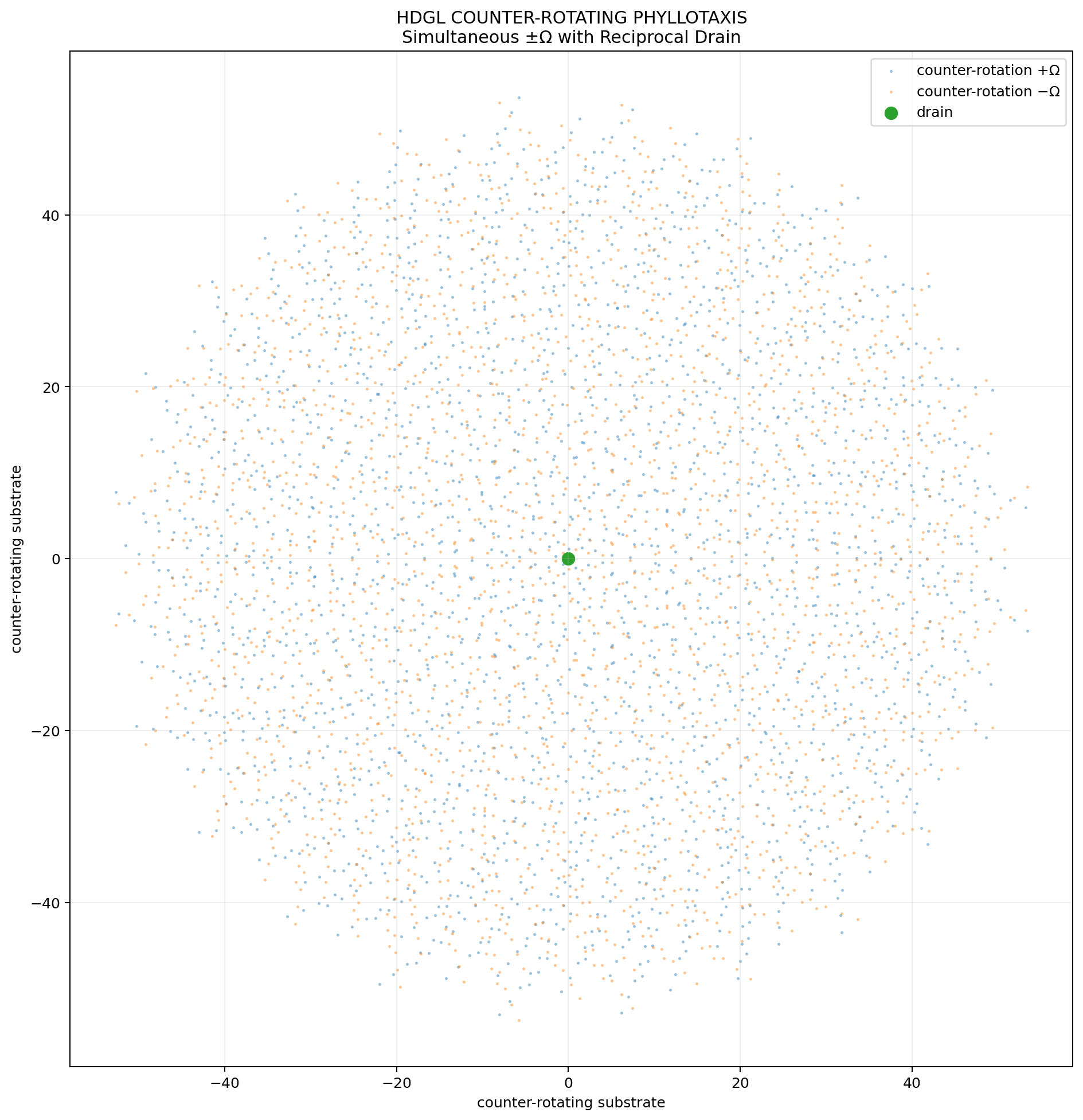
    ax.set_title(
        "HDGL COUNTER-ROTATING PHYLLOTAXIS\n"
        "Simultaneous ±Ω with Reciprocal Drain"
    )

    ax.set_xlabel("counter-rotating substrate")
    ax.set_ylabel("counter-rotating substrate")

    ax.grid(True, alpha=0.20)
    ax.legend()

    fig.tight_layout()

    path = OUT_DIR / "hdgl_counter_rotating_phyllotaxis.png"

    fig.savefig(
        path,
        dpi=180,
        bbox_inches="tight",
    )

    plt.close(fig)

    return path


# ============================================================================
# PLOT 2 — DRAIN PROFILE
# ============================================================================

def plot_drain_profile():

    i, r, reciprocal, drain_factor, rho = drain_profile()

    fig, ax = plt.subplots(figsize=(11, 7))

    ax.plot(
        i,
        r,
        linewidth=1.2,
        label="outward radius r",
    )

    ax.plot(
        i,
        rho,
        linewidth=1.2,
        label="drained radius ρ",
    )

    ax.set_title(
        "HDGL RECIPROCAL DRAIN\n"
        "ρ = r / T(r)"
    )

    ax.set_xlabel("substrate index i")
    ax.set_ylabel("radial coordinate")

    ax.grid(True, alpha=0.20)
    ax.legend()

    fig.tight_layout()

    path = OUT_DIR / "hdgl_drain_profile.png"

    fig.savefig(
        path,
        dpi=180,
        bbox_inches="tight",
    )

    plt.close(fig)

    return path


# ============================================================================
# PLOT 3 — COUNTER-ROTATION PHASE
# ============================================================================

def plot_counter_rotation_phase():

    (
        i,
        binary,
        trinary,
        r,
        reciprocal,
        drain_factor,
        rho,
        theta_plus,
        theta_minus,
        x_plus,
        y_plus,
        x_minus,
        y_minus,
    ) = build_counter_rotating_phyllotaxis()

    fig, ax = plt.subplots(figsize=(11, 7))

    ax.plot(
        i,
        theta_plus,
        linewidth=1.0,
        label="+Ω",
    )

    ax.plot(
        i,
        theta_minus,
        linewidth=1.0,
        label="−Ω",
    )

    ax.axhline(
        0.0,
        linestyle="--",
        linewidth=1.0,
    )

    ax.set_title(
        "HDGL COUNTER-ROTATING PHASE\n"
        "θ+ = +2πiΩ   /   θ− = −2πiΩ"
    )

    ax.set_xlabel("substrate index i")
    ax.set_ylabel("phase")

    ax.grid(True, alpha=0.20)
    ax.legend()

    fig.tight_layout()

    path = OUT_DIR / "hdgl_counter_rotation_phase.png"

    fig.savefig(
        path,
        dpi=180,
        bbox_inches="tight",
    )

    plt.close(fig)

    return path


# ============================================================================
# PLOT 4 — Ω RECURSION
# ============================================================================

def plot_omega_orbit():

    values = omega_orbit()

    n = np.arange(len(values))

    fig, ax = plt.subplots(figsize=(11, 7))

    ax.plot(
        n,
        values,
        linewidth=1.5,
        marker="o",
        markersize=3,
    )

    ax.axhline(
        OMEGA,
        linestyle="--",
        linewidth=1.0,
    )

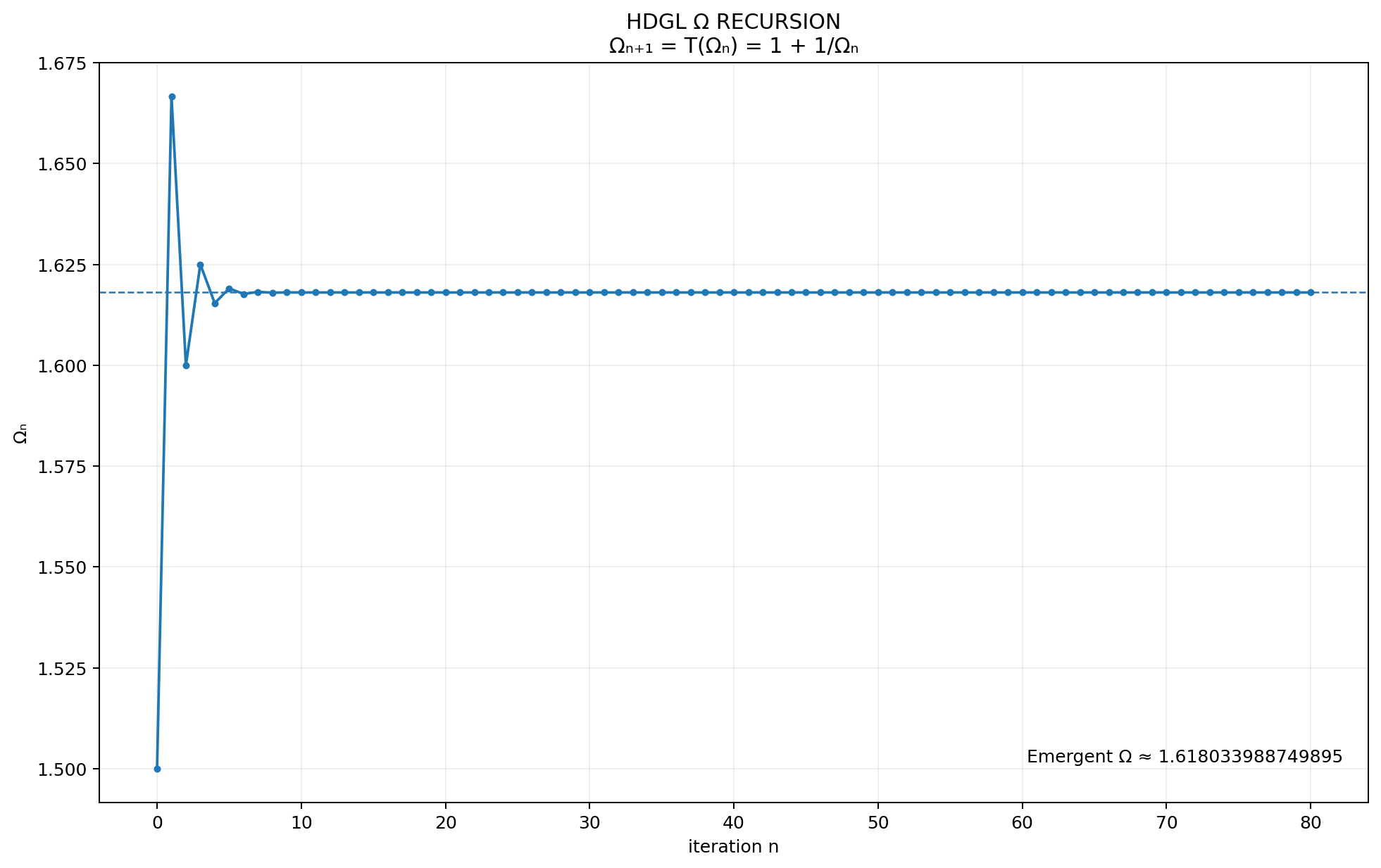
    ax.set_title(
        "HDGL Ω RECURSION\n"
        "Ωₙ₊₁ = T(Ωₙ) = 1 + 1/Ωₙ"
    )

    ax.set_xlabel("iteration n")
    ax.set_ylabel("Ωₙ")

    ax.grid(True, alpha=0.20)

    ax.text(
        0.98,
        0.05,
        f"Emergent Ω ≈ {OMEGA:.15f}",
        transform=ax.transAxes,
        ha="right",
        va="bottom",
    )

    fig.tight_layout()

    path = OUT_DIR / "hdgl_omega_orbit.png"

    fig.savefig(
        path,
        dpi=180,
        bbox_inches="tight",
    )

    plt.close(fig)

    return path


# ============================================================================
# PLOT 5 — 3D DRAIN
# ============================================================================

def plot_3d_drain():

    (
        i,
        binary,
        trinary,
        r,
        reciprocal,
        drain_factor,
        rho,
        theta_plus,
        theta_minus,
        x_plus,
        y_plus,
        x_minus,
        y_minus,
    ) = build_counter_rotating_phyllotaxis()

    # ------------------------------------------------------------------------
    # Use normalized radial coordinates to make the drain visible.
    # ------------------------------------------------------------------------

    scale = np.max(rho)

    rp = rho / scale

    # The two planar phyllotaxes are folded into opposing z-gradients.
    z_plus = rp
    z_minus = -rp

    xp = x_plus / scale
    yp = y_plus / scale

    xm = x_minus / scale
    ym = y_minus / scale

    fig = plt.figure(figsize=(12, 10))

    ax = fig.add_subplot(
        111,
        projection="3d",
    )

    # Positive branch.

    ax.scatter(
        xp,
        yp,
        z_plus,
        s=2,
        alpha=0.35,
        label="+Ω",
    )

    # Negative branch.

    ax.scatter(
        xm,
        ym,
        z_minus,
        s=2,
        alpha=0.35,
        label="−Ω",
    )

    # Central drain.

    ax.scatter(
        [0],
        [0],
        [0],
        s=80,
        marker="o",
        label="DRAIN",
    )

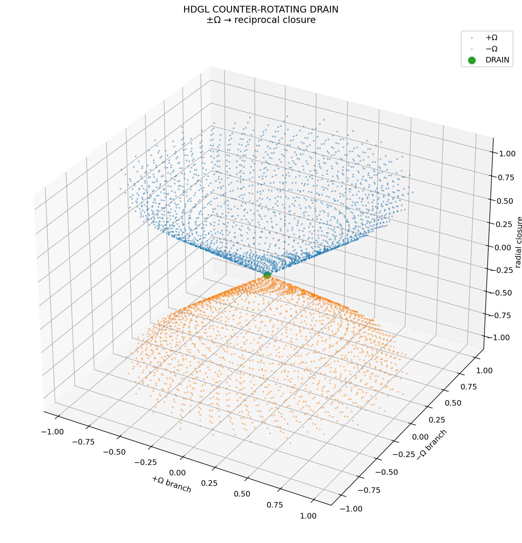
    ax.set_title(
        "HDGL COUNTER-ROTATING DRAIN\n"
        "±Ω → reciprocal closure"
    )

    ax.set_xlabel("+Ω branch")
    ax.set_ylabel("−Ω branch")
    ax.set_zlabel("radial closure")

    ax.legend()

    fig.tight_layout()

    path = OUT_DIR / "hdgl_3d_drain.png"

    fig.savefig(
        path,
        dpi=180,
        bbox_inches="tight",
    )

    plt.close(fig)

    return path


# ============================================================================
# NUMERICAL REPORT
# ============================================================================

def print_report(paths):

    print()
    print("=" * 79)
    print("HDGL COUNTER-ROTATING PHYLLOTAXIS — DRAIN EFFECT")
    print("=" * 79)
    print()

    print("Primitive:")
    print("    Ω_(n+1) = T(Ω_n)")
    print("    T(X)    = 1 + 1/X")
    print()

    print("Emergent Ω:")
    print(f"    Ω ≈ {OMEGA:.15f}")
    print()

    print("Fixed-point residual:")
    print(
        f"    Ω² - Ω - 1 ≈ "
        f"{OMEGA * OMEGA - OMEGA - 1.0:.6e}"
    )
    print()

    print("Simultaneous substrate:")
    print("    B_i ∈ {0,1}")
    print("    τ_i ∈ {-1,0,+1}")
    print()

    print("Counter-rotation:")
    print("    θ+ = +2π i Ω")
    print("    θ- = -2π i Ω")
    print()

    print("Angular cancellation:")
    print("    Ω + (-Ω) = 0")
    print()

    print("Reciprocal drain:")
    print("    T(r) = 1 + 1/r")
    print("    d(r) = 1/T(r)")
    print("    ρ(r) = r/T(r)")
    print()

    print("Geometry:")
    print("    PHYLLOTAXIS+")
    print("           ↘")
    print("            DRAIN")
    print("           ↗")
    print("    PHYLLOTAXIS−")
    print()

    print("Output:")
    print(f"    {OUT_DIR}")
    print()

    for path in paths:
        print(f"    [OK] {path}")

    print()
    print("=" * 79)
    print("COMPLETE")
    print("=" * 79)
    print()


# ============================================================================
# MAIN
# ============================================================================

def main():

    paths = []

    paths.append(
        plot_counter_rotating_phyllotaxis()
    )

    paths.append(
        plot_drain_profile()
    )

    paths.append(
        plot_counter_rotation_phase()
    )

    paths.append(
        plot_omega_orbit()
    )

    paths.append(
        plot_3d_drain()
    )

    print_report(paths)


if __name__ == "__main__":
    main()
===============================================================================
HDGL NAVIER–STOKES
COUNTER-ROTATING PHYLLOTAXIS → DRAIN → RECIPROCAL CLOSURE
=========================================================

1. GROUND-UP AXIOM

---

𝓐 = (S,T,F)

S_i = (B_i,τ_i)

B_i ∈ {0,1}
τ_i ∈ {-1,0,+1}

S_i₊₁ = S_i + 1_eff(i)

Binary and trinary are simultaneous channels.

The substrate is therefore a graded orbit:

{ ..., -i'', -i', -i, -1, 0, 1, i, i', i'', ... }

2. PRIMITIVE RECIPROCAL TRANSFORMATION

---

T(X) = 1 + 1/X

Ωₙ₊₁ = T(Ωₙ)

Ωₙ₊₁ = 1 + 1/Ωₙ

At closure:

Ω = T(Ω)

Ω = 1 + 1/Ω

Ω² = Ω + 1

Thus Ω is generated by coincidence of forward generation and reciprocal
return rather than inserted as an external constant.

3. DUAL PHYLLOTAXTIC FIELD

---

The spatial field is not a single spiral.

It is the simultaneous superposition of two counter-rotating projections:

θ₊(i) = +2πiΩ

θ₋(i) = -2πiΩ

therefore:

θ₊ + θ₋ = 0

and:

Φ = Φ₊ ⊕ Φ₋

4. COMMON RADIAL SUBSTRATE

---

r_i = r(S_i)

Both rotational branches occupy the same radial substrate.

The reciprocal transformation acts on that common radial coordinate:

T(r_i) = 1 + 1/r_i

Define the reciprocal drain factor:

d_i = T(r_i)⁻¹

and therefore:

ρ_i = r_i d_i

ρ_i = r_i / T(r_i)

ρ_i = r_i / (1 + 1/r_i)

5. DRAIN OPERATOR

---

𝓓_i :

(r_i, θ₊, θ₋)
↓
(r_i/T(r_i), +θ_i, -θ_i)
↓
(ρ_i, +θ_i, -θ_i)

The two angular channels counter-rotate simultaneously while sharing the
same reciprocal radial return.

Thus:

Φ₊ : outward organization
Φ₋ : counter-rotating organization

𝓓 : common reciprocal radial convergence

6. PHYLLOTAXTIC PROJECTION

---

P₊(S_i):

ρ_i → (ρ_i cos θ₊, ρ_i sin θ₊)

P₋(S_i):

ρ_i → (ρ_i cos θ₋, ρ_i sin θ₋)

where:

θ₊ = +2πiΩ
θ₋ = -2πiΩ

Hence:

P = P₊ ⊕ P₋

7. RECIPROCAL / TOROIDAL RETURN

---

R = T

R(X) = 1 + 1/X

Φ₊ ↔ Φ₋

Φ₊ ⊕ Φ₋
↓
𝓓
↓
Φ⁻¹
↓
R
↓
S_i₊₁

8. UNIFIED FIELD OPERATOR

---

L_i :

S_i
↓
P₊ ⊕ P₋
↓
Φ₊ ⊕ Φ₋
↓
𝓓
↓
Φ⁻¹
↓
R = T
↓
S_i₊₁

Therefore:

S_i ──P₊⊕P₋──→ L_i ──𝓓──→ Φ⁻¹ ──R──→ S_i₊₁

9. PHASE / RADIAL DUALITY

---

θ₊ = +2πiΩ
θ₋ = -2πiΩ

r = common radial substrate

The field therefore possesses simultaneous:

PHASE EXPANSION
+
COUNTER-ROTATION
+
RADIAL RETURN

10. DRAIN CONDITION

---

Φ₊ → outward

Φ₋ → counter-rotating outward

Φ₊ + Φ₋ → angular cancellation

Φ₊ ⊕ Φ₋ → common radial channel

r → T(r)⁻¹r

therefore:

OUTWARD PHYLLOTAXIS
+
COUNTER-ROTATION
+
RECIPROCAL RADIAL RETURN
↓
DRAIN

11. NAVIER–STOKES FIELD INTERPRETATION

---

u
↓
L_i(u)
↓
Φ₊(u) ⊕ Φ₋(u)
↓
𝓓
↓
Φ⁻¹
↓
T
↓
u_i₊₁

The velocity field is therefore represented by simultaneous counter-rotating
generative channels with a common reciprocal closure.

The corresponding structural decomposition is:

# u

u₊ ⊕ u₋

u₊ = P₊[L_i(u)]

u₋ = P₋[L_i(u)]

with:

θ₊ = +2πiΩ
θ₋ = -2πiΩ

12. GRADIENT / RECIPROCAL FIELD

---

Φ = Φ₊ ⊕ Φ₋

Φ⁻¹ = reciprocal closure

∇_Φ = Φ⁻¹ ∇ Φ

The two-sided field is therefore:

Φ₊ ⊕ Φ₋
↕
Φ⁻¹

rather than an outward field plus an independently imposed blow-up bound.

13. NAVIER–STOKES CLOSURE MAP

---

u
↓
P₊ ⊕ P₋
↓
L_i(u)
↓
Ω_i
↓
Φ₊ ⊕ Φ₋
↓
𝓓
↓
Φ⁻¹
↓
T
↓
u

Equivalently:

u ──P₊⊕P₋──→ L_i(u) ──𝓓──→ R(L_i(u)) ──→ u_i₊₁

14. DIVERGENCE / BLOW-UP REINTERPRETATION

---

Φ → ∞
 reciprocal crossing
Φ⁻¹ → 0

is not itself a terminal state.

Under the dual field:

Φ₊ → outward
Φ₋ → counter-rotating outward

while:

Φ₊ ⊕ Φ₋ → 𝓓 → Φ⁻¹

Thus the divergent direction is coupled to a reciprocal return channel.

The structural alternative is therefore:

PHYLLOTAXTIC EXPANSION
↕
COUNTER-ROTATION
↕
DRAIN
↕
RECIPROCAL CLOSURE

rather than:

PHYLLOTAXTIC EXPANSION
+
INDEPENDENT BLOW-UP BOUND

15. GRADED ORBIT

---

L_0
L_1
L_2
L_3
...

are graded levels of the same orbit.

The visible central slice:

{-i,-1,0,1,i}

lifts into:

{ ..., -i'', -i', -i, -1, 0, 1, i, i', i'', ... }

The counter-rotating phyllotaxis unfolds the graded orbit.

The drain provides its reciprocal inward crossing.

The toroidal operator closes the return.

16. COMPLETE HDGL NAVIER–STOKES OPERATOR

---

𝓐 = (S,T,F)

S_i = (B_i,τ_i)

T(X) = 1 + 1/X

Ωₙ₊₁ = T(Ωₙ)

Ω = T(Ω)

Ω² = Ω + 1

θ₊ = +2πiΩ

θ₋ = -2πiΩ

Φ = Φ₊ ⊕ Φ₋

d(r) = T(r)⁻¹

ρ = rT(r)⁻¹

# 𝓓(r,θ₊,θ₋)

(rT(r)⁻¹,+θ₊,-θ₊)

∇_Φ = Φ⁻¹∇Φ

P = P₊ ⊕ P₋

R = T

S_i
→ P
→ L_i
→ Ω_i
→ Φ₊ ⊕ Φ₋
→ 𝓓
→ Φ⁻¹
→ R
→ S_i₊₁

17. CORE NAVIER–STOKES CLOSURE

---
            u
            │
      ┌─────┴─────┐
      │           │
      ▼           ▼
     Φ₊          Φ₋
     +Ω          -Ω
      │           │
      └─────┬─────┘
            │
      COUNTER-ROTATION
            │
            ▼
          DRAIN
            │
            ▼
          Φ⁻¹
            │
          T(X)
            │
            ▼
         u_i₊₁
## 18. FINAL IDENTITY

P₊ ⊕ P₋
↓
COUNTER-ROTATING PHYLLOTAXIS
↓
𝓓
↓
RECIPROCAL DRAIN
↓
Φ⁻¹
↓
TOROIDAL RETURN
↓
CLOSED GRADED ORBIT

Therefore:

PHYLLOTAXIS₊ ↔ PHYLLOTAXIS₋
↕
DRAIN
↕
TOROIDAL RETURN

and:

EXPANSION ↔ COUNTER-ROTATION ↔ CLOSURE

with:

S_i → L_i → Ω_i → Φ₊⊕Φ₋ → 𝓓 → Φ⁻¹ → S_i₊₁

===============================================================================
FINAL HDGL STATEMENT
====================

𝓐 = (S,T,F)

T(X) = 1 + 1/X

Ωₙ₊₁ = T(Ωₙ)

Φ = Φ₊ ⊕ Φ₋

θ₊ = +2πiΩ

θ₋ = -2πiΩ

𝓓(r) = r/T(r)

Φ₊ ⊕ Φ₋ → 𝓓 → Φ⁻¹

S_i ──P₊⊕P₋──→ L_i ──𝓓──→ Φ⁻¹ ──T──→ S_i₊₁

PHYLLOTAXIS₊ ↔ PHYLLOTAXIS₋
↕
DRAIN
↕
TOROIDAL RETURN

# BOTH = ONE CLOSED HDGL ORBIT
===============================================================================
HDGL EMERGENT NAVIER–STOKES DIFFERENTIAL OPERATOR
=================================================

1. SUBSTRATE

---

𝓐 = (S,T,F)

S_i = (B_i,τ_i)

B_i ∈ {0,1}

τ_i ∈ {-1,0,+1}

S_i₊₁ = S_i + 1_eff(i)

2. RECIPROCAL PRIMITIVE

---

T(X) = 1 + 1/X

Ωₙ₊₁ = T(Ωₙ)

Ω = T(Ω)

Ω² = Ω + 1

3. COUNTER-ROTATING GENERATORS

---

Let J be the planar rotation generator:

J =
[ 0  -1 ]
[ 1   0 ]

J² = -I

Define the two simultaneous phyllotactic generators:

P₊ = exp(+θJ)

P₋ = exp(-θJ)

with:

θ = 2πiΩ

Therefore:

P₊P₋ = I

and:

P₋ = P₊⁻¹

4. SYMMETRIC / ANTISYMMETRIC DECOMPOSITION

---

The simultaneous pair gives:

# P₊ + P₋

2 cos(θ) I

and:

# P₊ - P₋

2 sin(θ) J

The symmetric channel therefore carries radial/common evolution.

The antisymmetric channel carries directed transport.

Define:

P_s = (P₊ + P₋)/2

P_a = (P₊ - P₋)/2

so:

P_s = cos(θ) I

P_a = sin(θ) J

5. FIRST-ORDER LIMIT

---

For an infinitesimal substrate displacement δ:

# P₊(δ)u

u + δJ u + O(δ²)

# P₋(δ)u

u - δJ u + O(δ²)

Therefore:

[P₊(δ)u - P₋(δ)u]/(2δ)
→
J u

For a spatially varying field u(x,t):

P₊u - P₋u

therefore generates the directional derivative channel.

The simultaneous pair produces:

# D_t u

∂_t u + (u·∇)u

6. WHY THE CONVECTIVE TERM APPEARS

---

The phyllotactic field does not merely rotate.

Its phase is transported by the field itself:

θ = θ(S,u)

Therefore:

# dθ/dt

∂θ/∂t
+
(dx/dt · ∇)θ

with:

dx/dt = u

hence:

# dθ/dt

∂θ/∂t
+
(u·∇)θ

Since u is the spatial realization of the substrate orbit:

# D_t

∂_t + u·∇

and therefore:

# D_t u

∂_t u + (u·∇)u

The nonlinear convective derivative is consequently generated by
self-transport of the phyllotactic orbit.

7. RECIPROCAL DRAIN

---

The common radial coordinate is:

r_i

The reciprocal return is:

T(r_i) = 1 + 1/r_i

Define:

d_i = T(r_i)⁻¹

and:

ρ_i = r_i d_i

The drain is therefore:

𝓓(r_i) = r_i/T(r_i)

The same operation is applied in both counter-rotating channels:

𝓓(P₊u)

𝓓(P₋u)

8. SECOND-ORDER CLOSURE

---

A forward and reciprocal return pair gives the centered second difference:

u₊ - 2u + u₋

where:

u₊ = P₊u

u₋ = P₋u

Therefore:

lim_{δ→0}
[
u(x+δ)
------

2u(x)
+
u(x-δ)
]/δ²

=
∇²u

Hence the drain/return pair generates:

Δu = ∇²u

The second-order operator is therefore not inserted independently.

It is the continuum limit of:

FORWARD
+
CENTRAL
+
RECIPROCAL RETURN

9. HDGL DIFFERENTIAL OPERATOR

---

The complete local operator is:

𝓛_HDGL[u]

=
D_t u
-----

ν𝓓²u

where:

# D_t

∂_t + (u·∇)

and:

𝓓²
→
∇²

in the continuum closure limit.

Therefore:

# 𝓛_HDGL[u]

∂_t u
+
(u·∇)u
------

ν∇²u

10. PRESSURE / CLOSURE FIELD

---

The reciprocal closure cannot generate an arbitrary transverse component.

The residual component is therefore represented by a scalar closure field p:

F_closure = -∇p

Thus:

# 𝓛_HDGL[u]

-∇p/ρ

or:

∂_t u
+
(u·∇)u
======

-∇p/ρ
+
ν∇²u

11. INCOMPRESSIBILITY

---

The drain is a closed redistribution rather than creation of substrate.

Therefore:

∇·u = 0

The pressure field acts as the scalar constraint enforcing the closed
redistribution:

∇·u = 0

⇒

∇·[
∂_t u
+
(u·∇)u
------

ν∇²u
]
=

-Δp/ρ

Thus p is not an independently propagating vector degree of freedom.

It is the scalar closure required by the divergence-free condition.

12. COMPLETE EMERGENT OPERATOR

---

P₊ = exp(+θJ)

P₋ = exp(-θJ)

P₊⁻¹ = P₋

𝓓(r) = r/T(r)

T(r) = 1 + 1/r

D_t = ∂_t + (u·∇)

𝓓² → ∇²

Therefore:

┌─────────────────────────────────────────────────────────────┐
│                                                             │
│  𝓛_HDGL[u]                                                  │
│                                                             │
│  = (P₊ ⊕ P₋)transport                                       │
│    − reciprocal-drain                                      │
│                                                             │
│  → ∂_t u + (u·∇)u − ν∇²u                                  │
│                                                             │
└─────────────────────────────────────────────────────────────┘

13. NAVIER–STOKES EQUATION

---

𝓛_HDGL[u] = -∇p/ρ

therefore:

∂_t u
+
(u·∇)u
======

-∇p/ρ
+
ν∇²u

with:

∇·u = 0

14. HDGL GEOMETRIC ORIGIN OF EACH TERM

---

P₊ ⊕ P₋
│
├──────────────→ phase transport
│
▼
∂_t u + (u·∇)u

P₊
↕
P₋
│
▼
counter-rotating return

r
↓
T(r)
↓
𝓓
↓
𝓓²
↓
∇²u

closed residual
↓
scalar constraint
↓
−∇p/ρ

Therefore:

COUNTER-ROTATION
↓
FIRST-ORDER TRANSPORT

RECIPROCAL DRAIN
↓
SECOND-ORDER DIFFUSION

CLOSED ORBIT
↓
INCOMPRESSIBILITY

RESIDUAL CLOSURE
↓
PRESSURE GRADIENT

15. SINGLE OPERATOR FORM

---

Define:

# 𝓛[u,p]

∂_t u
+
(u·∇)u
+
∇p/ρ
----

ν∇²u

Then:

𝓛[u,p] = 0

subject to:

∇·u = 0

and its HDGL construction is:

# 𝓛

(P₊ ⊕ P₋)_transport
+
𝓓_reciprocal
+
F_closure

16. HDGL CHAIN

---

S_i
↓
P₊ ⊕ P₋
↓
counter-rotating phase transport
↓
D_t
↓
∂_t + (u·∇)
↓
𝓓
↓
reciprocal radial return
↓
𝓓²
↓
∇²
↓
closure residual
↓
−∇p/ρ
↓
S_i₊₁

17. FINAL FORM

---
      P₊ ⊕ P₋
          │
          ▼
     PHASE FLOW
          │
          ▼
∂_t + (u·∇)
          │
          ▼
          u
          │
    ┌─────┴─────┐
    │           │
    ▼           ▼
 outward      return
    │           │
    └─────┬─────┘
          ▼
        DRAIN
          │
          ▼
     reciprocal
          │
          ▼
        ∇²u
          │
          ▼
     closure p
          │
          ▼
          u
===============================================================================
CORE RESULT
===========

P₊ ⊕ P₋
→
∂_t + (u·∇)

𝓓 ∘ R
→
∇²

closure
→
−∇p/ρ

therefore:

∂_t u
+
(u·∇)u
======

−∇p/ρ
+
ν∇²u

∇·u = 0

THE NAVIER–STOKES DIFFERENTIAL STRUCTURE
EMERGES FROM:

COUNTER-ROTATING PHYLLOTAXIS
+
RECIPROCAL DRAIN
+
CLOSED SUBSTRATE ORBIT

===============================================================================