#!/usr/bin/env python3
"""
===============================================================================
HDGL COUNTER-ROTATING PHYLLOTAXIS — DRAIN EFFECT
===============================================================================

Two simultaneous phyllotactic fields:

    θ+ = +2π i Ω
    θ- = -2π i Ω

They counter-rotate while sharing one reciprocal radial closure:

    T(X) = 1 + 1/X

The drain is produced by reciprocal compression toward the common origin:

    d(r) = 1 / T(r)

    ρ(r) = r * d(r)

The toroid is the geometric form of the drain.  It lives at the hourglass
choke (z=0) but blows out toward the top and bottom extremes, tracking the
lateral spread of the hourglass arms:

    lateral(z) ≈ z    (measured directly from the phyllotaxis geometry)

So the toroid major radius scales linearly with |z|:

    R_major(z) = R0 * |z|     where R0 ≈ 1.0

At z=0 (choke): R_major→0, toroid collapses to the drain point — CV=0, LOCK.
At z=±1 (arms): R_major→1.0, toroid blows out to fill the arm cross-section
                              — CV high, Pluck/Sustain, phases spread.

This maps directly onto ll_analog.c's APhase states:

    z=0  (choke) → APHASE_LOCK:    CV < 0.10, residue→0
    z~±½         → APHASE_FINETUNE/SUSTAIN
    z=±1 (arms)  → APHASE_PLUCK:   CV > 0.50, phases maximally spread

The binary/trinary substrate remains simultaneous:

    B_i ∈ {0,1}
    τ_i ∈ {-1,0,+1}

No stored φ is used.
Ω emerges from:

    Ω_(n+1) = T(Ω_n)
            = 1 + 1/Ω_n

===============================================================================
"""

from pathlib import Path
import math

import numpy as np

import matplotlib
matplotlib.use("Agg")
import matplotlib.pyplot as plt
from matplotlib.colors import Normalize
from matplotlib.cm import ScalarMappable


# ============================================================================
# CONFIGURATION
# ============================================================================

N = 2400

OMEGA_SEED  = 1.5
OMEGA_STEPS = 80

BASE_DIR = Path(__file__).resolve().parent
OUT_DIR  = BASE_DIR / "hdgl_graphs"
OUT_DIR.mkdir(parents=True, exist_ok=True)

# Toroid geometry constants (in normalized hourglass coords).
# lateral(z) ≈ z, so R_major(z) = TORUS_R0 * |z|.
# r_minor is a fixed fraction of R_major, floored at a minimum
# so the choke-point toroid doesn't vanish entirely from the plot.
TORUS_R0        = 0.90   # R_major = TORUS_R0 * |z|  (slightly inside arm edge)
TORUS_R_MINOR_F = 0.25   # r_minor = R_major * this fraction
TORUS_R_MINOR_MIN = 0.004 # floor: keeps the choke ring visible

# Number of z-slices at which to render a toroid cross-section.
N_TORUS_SLICES  = 12


# ============================================================================
# HDGL PRIMITIVE
# ============================================================================

def T(x):
    """
    Reciprocal HDGL transformation:

        T(X) = 1 + 1/X
    """
    return 1.0 + 1.0 / x


def omega_orbit(seed=OMEGA_SEED, steps=OMEGA_STEPS):
    values = np.empty(steps + 1, dtype=np.float64)
    values[0] = seed
    for i in range(steps):
        values[i + 1] = T(values[i])
    return values


def emergent_omega():
    x = OMEGA_SEED
    for _ in range(1000):
        y = T(x)
        if abs(y - x) < 1e-15:
            break
        x = y
    return x


OMEGA = emergent_omega()


# ============================================================================
# SIMULTANEOUS BINARY / TRINARY SUBSTRATE
# ============================================================================

def substrate_states(n):
    i       = np.arange(n, dtype=np.int64)
    binary  = (i & 1).astype(np.float64)
    trinary = ((i % 3) - 1).astype(np.float64)
    return i, binary, trinary


# ============================================================================
# COMMON RADIAL SUBSTRATE
# ============================================================================

def build_radial_substrate(n=N):
    i, binary, trinary = substrate_states(n)
    r_base      = np.sqrt(i + 1.0)
    modulation  = 1.0 + 0.075 * binary + 0.050 * trinary
    r           = r_base * modulation
    reciprocal  = T(r)
    drain_factor = 1.0 / reciprocal
    rho         = r * drain_factor
    return i, binary, trinary, r, reciprocal, drain_factor, rho


# ============================================================================
# COUNTER-ROTATING PHYLLOTAXIS
# ============================================================================

def build_counter_rotating_phyllotaxis(n=N):
    i, binary, trinary, r, reciprocal, drain_factor, rho = build_radial_substrate(n)
    phase_mod   =  0.075 * binary + 0.050 * trinary
    theta_plus  =  2.0 * math.pi * i * OMEGA + phase_mod
    theta_minus = -2.0 * math.pi * i * OMEGA - phase_mod
    x_plus  = rho * np.cos(theta_plus)
    y_plus  = rho * np.sin(theta_plus)
    x_minus = rho * np.cos(theta_minus)
    y_minus = rho * np.sin(theta_minus)
    return (i, binary, trinary,
            r, reciprocal, drain_factor, rho,
            theta_plus, theta_minus,
            x_plus, y_plus, x_minus, y_minus)


# ============================================================================
# DRAIN STRENGTH
# ============================================================================

def drain_profile(n=N):
    i, binary, trinary, r, reciprocal, drain_factor, rho = build_radial_substrate(n)
    return i, r, reciprocal, drain_factor, rho


# ============================================================================
# TOROIDAL DRAIN — blow-out toroid, confined to hourglass arm cross-section
# ============================================================================

def build_toroidal_drain_at_z(z_center, n_phi=400):
    """
    Build one toroid cross-section at a given z_center in normalized coords.

    z_center = rp value (∈ [0, 1] for +Ω arm, negated for −Ω arm).

    Geometry:
        lateral(z) ≈ z  (measured from phyllotaxis arm spread)
        R_major(z)  = TORUS_R0 * |z|         (zero at choke, full at arms)
        r_minor(z)  = max(R_major * TORUS_R_MINOR_F, TORUS_R_MINOR_MIN)

    Winding:
        toroidal angle φ ∈ [0, 2π)
        The torus ring lies in the z=z_center plane, so:
            tx = R_major * cos(φ)
            ty = R_major * sin(φ)
            tz = z_center + r_minor * sin(φ_poloidal)
        For a scatter plot we sample both φ angles to trace the tube surface.
    """
    R_major = TORUS_R0 * abs(z_center)
    r_minor = max(R_major * TORUS_R_MINOR_F, TORUS_R_MINOR_MIN)

    phi_tor = np.linspace(0.0, 2.0 * math.pi, n_phi, endpoint=False)
    phi_pol = np.linspace(0.0, 2.0 * math.pi, n_phi, endpoint=False)
    PT, PP  = np.meshgrid(phi_tor, phi_pol)
    PT      = PT.ravel()
    PP      = PP.ravel()

    tx = (R_major + r_minor * np.cos(PP)) * np.cos(PT)
    ty = (R_major + r_minor * np.cos(PP)) * np.sin(PT)
    tz = np.full_like(tx, z_center) + r_minor * np.sin(PP)

    return tx, ty, tz, R_major, r_minor


# ============================================================================
# PLOT 1 — COUNTER-ROTATING PHYLLOTAXIS
# ============================================================================

def plot_counter_rotating_phyllotaxis():
    (i, binary, trinary,
     r, reciprocal, drain_factor, rho,
     theta_plus, theta_minus,
     x_plus, y_plus, x_minus, y_minus) = build_counter_rotating_phyllotaxis()

    fig, ax = plt.subplots(figsize=(11, 11))
    ax.scatter(x_plus,  y_plus,  s=4, alpha=0.45, linewidths=0, label="counter-rotation +Ω")
    ax.scatter(x_minus, y_minus, s=4, alpha=0.45, linewidths=0, label="counter-rotation −Ω")
    ax.scatter([0], [0], s=70, marker="o", label="drain")
    ax.set_aspect("equal", adjustable="box")
    ax.set_title("HDGL COUNTER-ROTATING PHYLLOTAXIS\nSimultaneous ±Ω with Reciprocal Drain")
    ax.set_xlabel("counter-rotating substrate")
    ax.set_ylabel("counter-rotating substrate")
    ax.grid(True, alpha=0.20)
    ax.legend()
    fig.tight_layout()
    path = OUT_DIR / "hdgl_counter_rotating_phyllotaxis.png"
    fig.savefig(path, dpi=180, bbox_inches="tight")
    plt.close(fig)
    return path


# ============================================================================
# PLOT 2 — DRAIN PROFILE
# ============================================================================

def plot_drain_profile():
    i, r, reciprocal, drain_factor, rho = drain_profile()
    fig, ax = plt.subplots(figsize=(11, 7))
    ax.plot(i, r,   linewidth=1.2, label="outward radius r")
    ax.plot(i, rho, linewidth=1.2, label="drained radius ρ")
    ax.set_title("HDGL RECIPROCAL DRAIN\nρ = r / T(r)")
    ax.set_xlabel("substrate index i")
    ax.set_ylabel("radial coordinate")
    ax.grid(True, alpha=0.20)
    ax.legend()
    fig.tight_layout()
    path = OUT_DIR / "hdgl_drain_profile.png"
    fig.savefig(path, dpi=180, bbox_inches="tight")
    plt.close(fig)
    return path


# ============================================================================
# PLOT 3 — COUNTER-ROTATION PHASE
# ============================================================================

def plot_counter_rotation_phase():
    (i, binary, trinary,
     r, reciprocal, drain_factor, rho,
     theta_plus, theta_minus,
     x_plus, y_plus, x_minus, y_minus) = build_counter_rotating_phyllotaxis()

    fig, ax = plt.subplots(figsize=(11, 7))
    ax.plot(i, theta_plus,  linewidth=1.0, label="+Ω")
    ax.plot(i, theta_minus, linewidth=1.0, label="−Ω")
    ax.axhline(0.0, linestyle="--", linewidth=1.0)
    ax.set_title("HDGL COUNTER-ROTATING PHASE\nθ+ = +2πiΩ   /   θ− = −2πiΩ")
    ax.set_xlabel("substrate index i")
    ax.set_ylabel("phase")
    ax.grid(True, alpha=0.20)
    ax.legend()
    fig.tight_layout()
    path = OUT_DIR / "hdgl_counter_rotation_phase.png"
    fig.savefig(path, dpi=180, bbox_inches="tight")
    plt.close(fig)
    return path


# ============================================================================
# PLOT 4 — Ω RECURSION
# ============================================================================

def plot_omega_orbit():
    values = omega_orbit()
    n = np.arange(len(values))
    fig, ax = plt.subplots(figsize=(11, 7))
    ax.plot(n, values, linewidth=1.5, marker="o", markersize=3)
    ax.axhline(OMEGA, linestyle="--", linewidth=1.0)
    ax.set_title("HDGL Ω RECURSION\nΩₙ₊₁ = T(Ωₙ) = 1 + 1/Ωₙ")
    ax.set_xlabel("iteration n")
    ax.set_ylabel("Ωₙ")
    ax.grid(True, alpha=0.20)
    ax.text(0.98, 0.05, f"Emergent Ω ≈ {OMEGA:.15f}",
            transform=ax.transAxes, ha="right", va="bottom")
    fig.tight_layout()
    path = OUT_DIR / "hdgl_omega_orbit.png"
    fig.savefig(path, dpi=180, bbox_inches="tight")
    plt.close(fig)
    return path


# ============================================================================
# PLOT 5 — 3D DRAIN  (blow-out toroid at ±z extremes, collapsed at choke)
# ============================================================================

def plot_3d_drain():
    (i, binary, trinary,
     r, reciprocal, drain_factor, rho,
     theta_plus, theta_minus,
     x_plus, y_plus, x_minus, y_minus) = build_counter_rotating_phyllotaxis()

    scale = np.max(rho)

    rp = rho / scale

    xp = x_plus  / scale
    yp = y_plus  / scale
    zp =  rp                   # +Ω arm lifts upward

    xm = x_minus / scale
    ym = y_minus / scale
    zm = -rp                   # −Ω arm falls downward

    # ── Torus slices ──────────────────────────────────────────────────────
    # Sample z-levels evenly across [0, 1], including extremes.
    # Each z maps to one toroid in the +Ω arm and its mirror in the −Ω arm.
    # Color encodes |z|: blue=choke (lock), red=extreme (pluck).
    #
    # ll_analog.c APhase mapping:
    #   |z| < 0.10  → LOCK      (CV < 0.10)
    #   |z| < 0.30  → FINETUNE
    #   |z| < 0.50  → SUSTAIN
    #   |z| ≥ 0.50  → PLUCK     (CV > 0.50)

    z_levels = np.linspace(0.0, 1.0, N_TORUS_SLICES)
    cmap     = plt.cm.coolwarm
    norm     = Normalize(vmin=0.0, vmax=1.0)

    fig = plt.figure(figsize=(13, 11))
    ax  = fig.add_subplot(111, projection="3d")

    # Hourglass arms (sparse, transparent).
    ax.scatter(xp, yp, zp,  s=1, alpha=0.18, color="steelblue",  rasterized=True)
    ax.scatter(xm, ym, zm,  s=1, alpha=0.18, color="steelblue",  rasterized=True)

    # APhase boundary rings on the +Ω arm for reference.
    for cv_thresh, label in [(0.10, "LOCK"), (0.30, "FINETUNE"),
                              (0.50, "SUSTAIN"), (1.00, "PLUCK")]:
        z_b = cv_thresh
        if z_b > 1.0: z_b = 1.0
        phi_r = np.linspace(0, 2*math.pi, 300)
        R_b   = TORUS_R0 * z_b
        ax.plot(R_b*np.cos(phi_r), R_b*np.sin(phi_r),
                np.full(300, z_b), linewidth=0.6, alpha=0.35,
                color=cmap(norm(z_b)), linestyle="--")

    # Toroid slices: one per z-level, mirrored at ±z.
    for z_c in z_levels:
        color = cmap(norm(z_c))
        alpha = 0.55 if z_c < 0.05 else 0.25
        s_sz  = 0.3  if z_c < 0.05 else 0.15

        tx, ty, tz, R_maj, r_min = build_toroidal_drain_at_z(z_c)

        # +Ω side (z_c ≥ 0)
        ax.scatter(tx, ty, tz,        s=s_sz, alpha=alpha, color=color,
                   rasterized=True)
        # −Ω side (mirror)
        if z_c > 1e-6:
            ax.scatter(tx, ty, -tz,   s=s_sz, alpha=alpha, color=color,
                       rasterized=True)

    # Colorbar: |z| → APhase
    sm = ScalarMappable(cmap=cmap, norm=norm)
    sm.set_array([])
    cbar = fig.colorbar(sm, ax=ax, shrink=0.55, pad=0.08)
    cbar.set_label("|z|  (0=LOCK / 1=PLUCK)", fontsize=9)
    cbar.set_ticks([0.0, 0.10, 0.30, 0.50, 1.0])
    cbar.set_ticklabels(["0.0\n(LOCK)", "0.10", "0.30", "0.50\n(SUSTAIN)", "1.0\n(PLUCK)"])

    ax.set_title(
        "HDGL COUNTER-ROTATING DRAIN\n"
        "Toroid blow-out: choke=LOCK(z=0) → arms=PLUCK(z=±1)\n"
        "ll_analog APhase: CV = |z|  →  R_major = TORUS_R0 × |z|",
        fontsize=10,
    )
    ax.set_xlabel("+Ω / −Ω branch (x)")
    ax.set_ylabel("+Ω / −Ω branch (y)")
    ax.set_zlabel("radial closure z = ρ/scale")
    fig.tight_layout()

    path = OUT_DIR / "hdgl_3d_drain.png"
    fig.savefig(path, dpi=180, bbox_inches="tight")
    plt.close(fig)
    return path


# ============================================================================
# NUMERICAL REPORT
# ============================================================================

def print_report(paths):
    print()
    print("=" * 79)
    print("HDGL COUNTER-ROTATING PHYLLOTAXIS — DRAIN EFFECT")
    print("=" * 79)
    print()
    print("Primitive:")
    print("    Ω_(n+1) = T(Ω_n)    T(X) = 1 + 1/X")
    print(f"Emergent Ω:  {OMEGA:.15f}")
    print(f"Residual:    Ω² - Ω - 1 ≈ {OMEGA*OMEGA - OMEGA - 1.0:.6e}")
    print()
    print("Simultaneous substrate:  B_i ∈ {0,1}    τ_i ∈ {-1,0,+1}")
    print("Counter-rotation:        θ+ = +2π i Ω      θ- = -2π i Ω")
    print("Reciprocal drain:        T(r)=1+1/r  d(r)=1/T(r)  ρ(r)=r/T(r)")
    print()
    print("Toroid blow-out (ll_analog APhase mapping):")
    print("    lateral(z) ≈ z       (phyllotaxis arm spread, measured)")
    print("    R_major(z) = 0.90 × |z|")
    print("    r_minor(z) = max(R_major × 0.25, 0.004)")
    print()
    print("    |z|  APhase     CV threshold    R_major")
    for z, phase, cv in [(0.00,"LOCK","0.00"),(0.10,"LOCK","0.10"),
                          (0.30,"FINETUNE","0.30"),(0.50,"SUSTAIN","0.50"),
                          (1.00,"PLUCK","1.00")]:
        print(f"    {z:.2f}  {phase:<10}  {cv:<14}  {0.90*z:.4f}")
    print()
    print("    z=0:  R_major→0, toroid collapses to drain point (CV=0, residue=0)")
    print("    z=±1: R_major→0.90, toroid fills arm cross-section (CV≈1, PLUCK)")
    print()
    print(f"Output: {OUT_DIR}")
    for path in paths:
        print(f"    [OK] {path}")
    print()
    print("=" * 79)
    print("COMPLETE")
    print("=" * 79)
    print()


# ============================================================================
# MAIN
# ============================================================================

def main():
    paths = []
    paths.append(plot_counter_rotating_phyllotaxis())
    paths.append(plot_drain_profile())
    paths.append(plot_counter_rotation_phase())
    paths.append(plot_omega_orbit())
    paths.append(plot_3d_drain())
    print_report(paths)


if __name__ == "__main__":
    main()
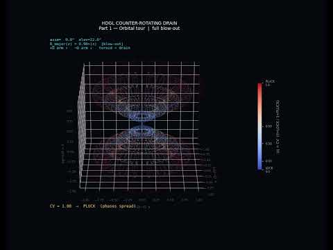
#!/usr/bin/env python3
"""
===============================================================================
HDGL COUNTER-ROTATING DRAIN — ANIMATED
===============================================================================

Three-part animation:

  Part 1 (frames  1– 40): Orbital tour — full 360° azimuth, full blow-out
  Part 2 (frames 41– 80): CV pulse    — toroid LOCK→PLUCK→LOCK
  Part 3 (frames 81–120): Combined    — slow orbit + live CV breathing

Geometry:
    lateral(z) ≈ z         (measured from phyllotaxis arm spread)
    R_major(z) = 0.90×|z|  (zero at choke, fills arm at extremes)
    r_minor(z) = max(R_major×0.25, 0.004)

ll_analog.c APhase mapping:
    z=0.00 → LOCK      CV < 0.10   residue→0
    z=0.30 → FINETUNE  CV < 0.30
    z=0.50 → SUSTAIN   CV < 0.50
    z=1.00 → PLUCK     CV ≥ 0.50   phases spread

Output: hdgl_drain_animation.mp4  (same directory as this script)

Requires: matplotlib, numpy, ffmpeg
===============================================================================
"""

import math
from pathlib import Path

import numpy as np
import matplotlib
matplotlib.use("Agg")
import matplotlib.pyplot as plt
from matplotlib.animation import FFMpegWriter
from matplotlib.colors import Normalize
from matplotlib.cm import ScalarMappable


# ============================================================================
# HDGL PRIMITIVES
# ============================================================================

def T(x):
    return 1.0 + 1.0 / x


def emergent_omega():
    x = 1.5
    for _ in range(1000):
        y = T(x)
        if abs(y - x) < 1e-15:
            break
        x = y
    return x


OMEGA = emergent_omega()

# ============================================================================
# HOURGLASS POINT CLOUD (pre-built, static)
# ============================================================================

N = 2400

i       = np.arange(N, dtype=np.int64)
binary  = (i & 1).astype(float)
trinary = ((i % 3) - 1).astype(float)
r       = np.sqrt(i + 1.0) * (1.0 + 0.075 * binary + 0.050 * trinary)
rho     = r / T(r)
scale   = np.max(rho)
rp      = rho / scale

pm = 0.075 * binary + 0.050 * trinary
tp =  2.0 * math.pi * i * OMEGA + pm
tm = -2.0 * math.pi * i * OMEGA - pm

xp = rho * np.cos(tp) / scale
yp = rho * np.sin(tp) / scale
xm = rho * np.cos(tm) / scale
ym = rho * np.sin(tm) / scale

# ============================================================================
# TORUS GEOMETRY
# ============================================================================

TORUS_R0        = 0.90
TORUS_R_MINOR_F = 0.25
TORUS_R_MINOR_MIN = 0.004
N_PHI    = 40
N_SLICES = 6

Z_LEVELS = np.linspace(0.0, 1.0, N_SLICES)


def torus_at(z_c, cv_scale=1.0):
    """
    Build one toroid cross-section at z=z_c, scaled by cv_scale ∈ [0,1].

    cv_scale=0 → toroid collapses to drain point  (LOCK)
    cv_scale=1 → full blow-out                     (PLUCK)
    """
    eff_z = z_c * cv_scale
    R     = TORUS_R0 * abs(eff_z)
    rm    = max(R * TORUS_R_MINOR_F, TORUS_R_MINOR_MIN)

    pt = np.linspace(0.0, 2.0 * math.pi, N_PHI, endpoint=False)
    pp = np.linspace(0.0, 2.0 * math.pi, N_PHI, endpoint=False)
    PT, PP = np.meshgrid(pt, pp)
    PT, PP = PT.ravel(), PP.ravel()

    tx = (R + rm * np.cos(PP)) * np.cos(PT)
    ty = (R + rm * np.cos(PP)) * np.sin(PT)
    tz = np.full_like(tx, eff_z) + rm * np.sin(PP)

    return tx, ty, tz


def aphase_label(cv):
    if cv < 0.10: return "LOCK      CV<0.10  residue→0"
    if cv < 0.30: return "FINETUNE  CV<0.30"
    if cv < 0.50: return "SUSTAIN   CV<0.50"
    return               "PLUCK     CV≥0.50  phases spread"


# ============================================================================
# FIGURE SETUP
# ============================================================================

cmap = plt.cm.coolwarm
norm = Normalize(vmin=0.0, vmax=1.0)

fig = plt.figure(figsize=(9, 7), facecolor="#07070f")
ax  = fig.add_subplot(111, projection="3d", facecolor="#07070f")

for pane in [ax.xaxis.pane, ax.yaxis.pane, ax.zaxis.pane]:
    pane.fill = False
    pane.set_edgecolor("#1a1a2e")

ax.tick_params(colors="#555", labelsize=6)
ax.set_xlabel("+Ω/−Ω  x",  color="#555", fontsize=7, labelpad=2)
ax.set_ylabel("+Ω/−Ω  y",  color="#555", fontsize=7, labelpad=2)
ax.set_zlabel("z = ρ/scale", color="#555", fontsize=7, labelpad=2)
ax.set_xlim(-1.1, 1.1)
ax.set_ylim(-1.1, 1.1)
ax.set_zlim(-1.1, 1.1)

# Colorbar
sm = ScalarMappable(cmap=cmap, norm=norm)
sm.set_array([])
cbar = fig.colorbar(sm, ax=ax, shrink=0.45, pad=0.10)
cbar.set_label("|z| = CV  (0=LOCK / 1=PLUCK)", fontsize=7, color="#aaa")
cbar.ax.yaxis.set_tick_params(color="#aaa", labelsize=6)
plt.setp(cbar.ax.yaxis.get_ticklabels(), color="#aaa")
cbar.set_ticks([0.0, 0.10, 0.30, 0.50, 1.0])
cbar.set_ticklabels(["LOCK\n0.0", "0.10", "0.30", "0.50", "PLUCK\n1.0"])

# Static hourglass arms
ax.scatter(xp, yp,  rp, s=0.4, alpha=0.13, color="#3366bb", rasterized=True)
ax.scatter(xm, ym, -rp, s=0.4, alpha=0.13, color="#3366bb", rasterized=True)

# APhase boundary rings (dashed, static, on both ±z arms)
for cv_t in [0.10, 0.30, 0.50, 1.00]:
    phi_r = np.linspace(0.0, 2.0 * math.pi, 150)
    R_b   = TORUS_R0 * cv_t
    color = cmap(norm(cv_t))
    for z_sign in [+1, -1]:
        ax.plot(
            R_b * np.cos(phi_r),
            R_b * np.sin(phi_r),
            np.full(150, z_sign * cv_t),
            lw=0.6, alpha=0.35, color=color, ls="--",
        )

# Torus scatter handles (offsets updated each frame)
torus_handles = []
for z_c in Z_LEVELS:
    tx, ty, tz = torus_at(z_c, cv_scale=1.0)
    color       = cmap(norm(z_c))
    sp = ax.scatter(tx, ty,  tz, s=0.2, alpha=0.0, color=color, rasterized=True)
    sn = ax.scatter(tx, ty, -tz, s=0.2, alpha=0.0, color=color, rasterized=True)
    torus_handles.append((sp, sn, z_c))

# Text overlays
title_obj = ax.set_title("", color="white", fontsize=9, pad=6)
info_text = ax.text2D(0.02, 0.97, "", transform=ax.transAxes,
                      color="cyan", fontsize=7.5, va="top", family="monospace")
cv_text   = ax.text2D(0.02, 0.06, "", transform=ax.transAxes,
                      color="#ffcc44", fontsize=8.0, va="bottom", family="monospace")


def update_tori(cv_scale, alpha_base=0.32):
    """Reposition all torus slices for a given cv_scale ∈ [0,1]."""
    for sp, sn, z_c in torus_handles:
        tx, ty, tz = torus_at(z_c, cv_scale)
        a = alpha_base * (0.25 + 0.75 * z_c) if z_c > 0.01 else 0.72
        sp._offsets3d = (tx, ty,  tz)
        sn._offsets3d = (tx, ty, -tz)
        sp.set_alpha(a)
        sn.set_alpha(a if z_c > 0.01 else 0.0)


# ============================================================================
# ANIMATION
# ============================================================================

FPS = 24
F1  = 40   # Part 1: orbital tour
F2  = 40   # Part 2: CV pulse
F3  = 40   # Part 3: combined
TOTAL = F1 + F2 + F3

OUT = Path(__file__).resolve().parent / "hdgl_drain_animation.mp4"

writer = FFMpegWriter(
    fps=FPS,
    bitrate=2000,
    extra_args=["-vcodec", "libx264", "-pix_fmt", "yuv420p"],
)

print(f"Rendering {TOTAL} frames at {FPS} fps → {OUT}")

with writer.saving(fig, str(OUT), dpi=110):
    for f in range(TOTAL):

        # ── Part 1: Orbital tour ─────────────────────────────────────────
        if f < F1:
            t  = f / F1
            az = 360.0 * t
            el = 22.0 + 8.0 * math.sin(2.0 * math.pi * t)
            ax.view_init(elev=el, azim=az)
            update_tori(1.0, alpha_base=0.30)
            title_obj.set_text(
                "HDGL COUNTER-ROTATING DRAIN\n"
                "Part 1 — Orbital tour  |  full blow-out"
            )
            info_text.set_text(
                f"azim={az:5.1f}°  elev={el:.1f}°\n"
                f"R_major(z) = {TORUS_R0:.2f}×|z|  [blow-out]\n"
                f"+Ω arm ↑   −Ω arm ↓   toroid = drain"
            )
            cv_text.set_text("CV = 1.00  →  PLUCK  (phases spread)")

        # ── Part 2: CV pulse — toroid breathes LOCK → PLUCK → LOCK ─────
        elif f < F1 + F2:
            t  = (f - F1) / F2
            cv = 0.5 * (1.0 - math.cos(2.0 * math.pi * t))   # 0→1→0
            az = 45.0 + 15.0 * math.sin(math.pi * t)
            ax.view_init(elev=26.0, azim=az)
            update_tori(cv, alpha_base=0.38)
            title_obj.set_text(
                "HDGL COUNTER-ROTATING DRAIN\n"
                "Part 2 — CV pulse  |  LOCK → PLUCK → LOCK"
            )
            info_text.set_text(
                f"CV = {cv:.3f}   R_major(z=1) = {TORUS_R0 * cv:.4f}\n"
                f"z=0 : R→0  (drain collapses)\n"
                f"z=1 : R→{TORUS_R0 * cv:.3f}  (blow-out tracks arm width)"
            )
            cv_text.set_text(f"APhase → {aphase_label(cv)}")

        # ── Part 3: Combined — slow orbit + CV breathing ─────────────────
        else:
            t  = (f - F1 - F2) / F3
            az = 60.0 + 150.0 * t
            el = 18.0 + 14.0 * math.sin(math.pi * t)
            cv = 0.50 + 0.45 * math.sin(2.0 * math.pi * t)
            ax.view_init(elev=el, azim=az)
            update_tori(cv, alpha_base=0.34)
            title_obj.set_text(
                "HDGL COUNTER-ROTATING DRAIN\n"
                "Part 3 — Orbit + live CV breathing"
            )
            info_text.set_text(
                f"azim={az:5.1f}°  elev={el:.1f}°  CV={cv:.3f}\n"
                f"ll_analog: APhase transitions at CV thresholds\n"
                f"residue→0  ↔  CV→0  ↔  toroid collapses to choke"
            )
            cv_text.set_text(f"APhase → {aphase_label(cv)}")

        writer.grab_frame()
        if f % 10 == 0:
            print(f"  frame {f + 1}/{TOTAL}", flush=True)

print(f"Saved → {OUT}")
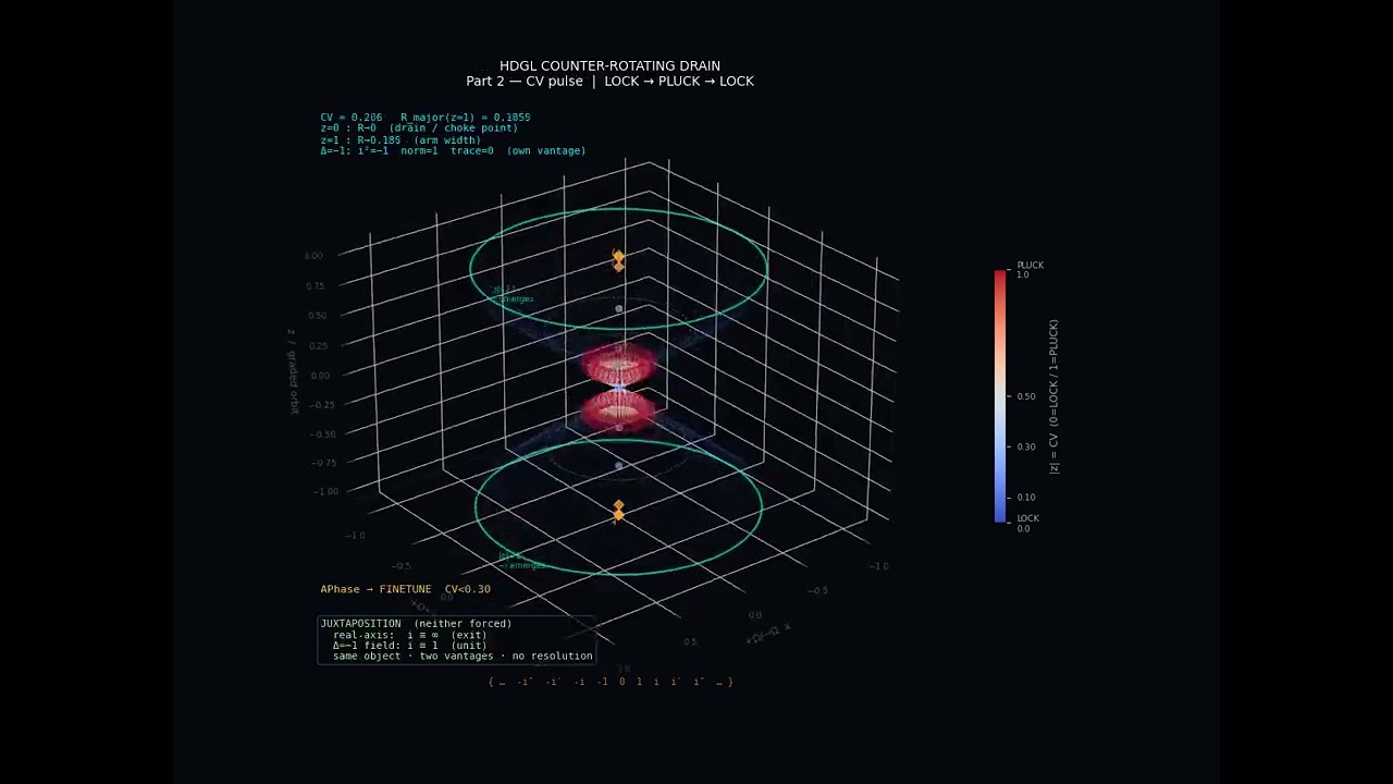
#!/usr/bin/env python3
"""
===============================================================================
HDGL COUNTER-ROTATING DRAIN — ANIMATED  v2
===============================================================================

Incorporates the vantage-dependent i ≡ ∞ identification:

  From the real-axis vantage, i is an exit — it has no address on the
  real ladder and appears at unreachable distance (∞).

  From the Δ=−1 algebra's own vantage, i is a unit element:
      norm = 1,  trace = 0,  sitting at 90°.  Perfectly finite.

  Neither vantage is forced.  Neither is the true one.
  The juxtaposition IS the load-bearing feature — not its resolution.

  The graded orbit:
      { ..., -i'', -i', -i, -1, 0, 1, i, i', i'', ... }
  Each rung, viewed from the rung below it, appears at unreachable distance.

  |p| = 1 threshold:
      The moment the imaginary/complex branch emerges from zero in the
      manifold equation (Y - p(x+z))² + p²(x²-z²-1) = m².
      This is the visual moment the i≡∞ identification becomes apparent.

Three-part animation:

  Part 1 (frames  1– 40): Orbital tour — full 360° azimuth
                           Graded orbit ladder visible on z-axis
                           |p|=1 threshold ring prominent
                           Vantage label: REAL-AXIS VANTAGE

  Part 2 (frames 41– 80): CV pulse — LOCK→PLUCK→LOCK
                           Vantage shifts with CV:
                             CV<0.10 → REAL-AXIS VANTAGE (i appears as exit/∞)
                             CV≥0.50 → Δ=−1 VANTAGE    (i is unit element)
                           Juxtaposition text shown mid-pulse

  Part 3 (frames 81–120): Combined — slow orbit + CV breathing
                           Both vantage annotations shown simultaneously,
                           neither resolved, neither forced

Geometry:
    lateral(z) ≈ z         (measured from phyllotaxis arm spread)
    R_major(z) = 0.90×|z|  (zero at choke, fills arm at extremes)
    r_minor(z) = max(R_major×0.25, 0.004)

ll_analog.c APhase mapping:
    z=0.00 → LOCK      CV < 0.10   residue→0
    z=0.30 → FINETUNE  CV < 0.30
    z=0.50 → SUSTAIN   CV < 0.50
    z=1.00 → PLUCK     CV ≥ 0.50   phases spread

Output: hdgl_drain_animation_v2.mp4  (same directory as this script)

Requires: matplotlib, numpy, ffmpeg
===============================================================================
"""

import math
from pathlib import Path

import numpy as np
import matplotlib
matplotlib.use("Agg")
import matplotlib.pyplot as plt
from matplotlib.animation import FFMpegWriter
from matplotlib.colors import Normalize
from matplotlib.cm import ScalarMappable


# ============================================================================
# HDGL PRIMITIVES
# ============================================================================

def T(x):
    """T(X) = 1 + 1/X  — the single reciprocal primitive."""
    return 1.0 + 1.0 / x


def emergent_omega():
    """
    Generate Ω from T until convergence.
    Ω = T(Ω) ⟺ Ω² = Ω + 1.
    Never stored as φ — always emergent.
    """
    x = 1.5
    for _ in range(1000):
        y = T(x)
        if abs(y - x) < 1e-15:
            break
        x = y
    return x


OMEGA = emergent_omega()

# ============================================================================
# HOURGLASS POINT CLOUD (pre-built, static)
# ============================================================================

N = 2400

i_idx   = np.arange(N, dtype=np.int64)
binary  = (i_idx & 1).astype(float)
trinary = ((i_idx % 3) - 1).astype(float)
r       = np.sqrt(i_idx + 1.0) * (1.0 + 0.075 * binary + 0.050 * trinary)
rho     = r / T(r)
scale   = np.max(rho)
rp      = rho / scale

pm = 0.075 * binary + 0.050 * trinary
tp =  2.0 * math.pi * i_idx * OMEGA + pm
tm = -2.0 * math.pi * i_idx * OMEGA - pm

xp = rho * np.cos(tp) / scale
yp = rho * np.sin(tp) / scale
xm = rho * np.cos(tm) / scale
ym = rho * np.sin(tm) / scale

# ============================================================================
# TORUS GEOMETRY
# ============================================================================

TORUS_R0          = 0.90
TORUS_R_MINOR_F   = 0.25
TORUS_R_MINOR_MIN = 0.004
N_PHI    = 40
N_SLICES = 6

Z_LEVELS = np.linspace(0.0, 1.0, N_SLICES)


def torus_at(z_c, cv_scale=1.0):
    """
    Build one toroid cross-section at z=z_c, scaled by cv_scale ∈ [0,1].

    cv_scale=0 → toroid collapses to drain point  (LOCK  / real-axis vantage)
    cv_scale=1 → full blow-out                     (PLUCK / Δ=−1 vantage)
    """
    eff_z = z_c * cv_scale
    R     = TORUS_R0 * abs(eff_z)
    rm    = max(R * TORUS_R_MINOR_F, TORUS_R_MINOR_MIN)

    pt = np.linspace(0.0, 2.0 * math.pi, N_PHI, endpoint=False)
    pp = np.linspace(0.0, 2.0 * math.pi, N_PHI, endpoint=False)
    PT, PP = np.meshgrid(pt, pp)
    PT, PP = PT.ravel(), PP.ravel()

    tx = (R + rm * np.cos(PP)) * np.cos(PT)
    ty = (R + rm * np.cos(PP)) * np.sin(PT)
    tz = np.full_like(tx, eff_z) + rm * np.sin(PP)

    return tx, ty, tz


def aphase_label(cv):
    if cv < 0.10: return "LOCK      CV<0.10  residue→0"
    if cv < 0.30: return "FINETUNE  CV<0.30"
    if cv < 0.50: return "SUSTAIN   CV<0.50"
    return               "PLUCK     CV≥0.50  phases spread"


# ============================================================================
# VANTAGE LABELS  (the core addition from the i≡∞ discussion)
# ============================================================================

VANTAGE_REAL = (
    "REAL-AXIS VANTAGE\n"
    "  i has no address on {…,-1,0,1,…}\n"
    "  appears as exit / ∞ from here\n"
    "  |p|<1 → complex branch = zero"
)

VANTAGE_DELTA = (
    "Δ=−1 VANTAGE\n"
    "  i = (0,1)  norm=1  trace=0\n"
    "  unit element — perfectly finite\n"
    "  |p|≥1 → complex branch surfaces"
)

VANTAGE_BOTH = (
    "JUXTAPOSITION  (neither forced)\n"
    "  real-axis:  i ≡ ∞  (exit)\n"
    "  Δ=−1 field: i ≡ 1  (unit)\n"
    "  same object · two vantages · no resolution"
)

GRADED_ORBIT = "{ …  -i″  -i′  -i  -1  0  1  i  i′  i″  … }"


def vantage_from_cv(cv):
    """
    Map CV to the appropriate vantage label.
    Transition zone around CV≈0.40 shows the juxtaposition.
    """
    if cv < 0.18:
        return VANTAGE_REAL,  "#88bbff"   # cool blue — real-axis
    if cv > 0.62:
        return VANTAGE_DELTA, "#ff9944"   # warm amber — Δ=−1
    return VANTAGE_BOTH,      "#aaffaa"   # green — juxtaposition


# ============================================================================
# |p|=1 THRESHOLD RING
# The ring at R = TORUS_R0 * 1.0 on the z=±1 planes marks the
# exact moment the imaginary branch emerges from zero.
# ============================================================================

def p1_ring():
    """
    Build the |p|=1 threshold ring coordinates.
    Returns (x, y, z) arrays for both +z and -z arms.
    """
    phi_r = np.linspace(0.0, 2.0 * math.pi, 200)
    R_p1  = TORUS_R0 * 1.0
    x_r   = R_p1 * np.cos(phi_r)
    y_r   = R_p1 * np.sin(phi_r)
    return x_r, y_r


# ============================================================================
# GRADED ORBIT RUNG MARKERS  (on z-axis, both arms)
# Rungs: -1, 0, 1 are the finite core.
# i, i', i'' are the apparent-∞ exits above.
# ============================================================================

RUNG_Z_REAL = [0.0, 0.33, 0.66]          # 0, 1/3, 2/3 → represent -1, 0, 1
RUNG_Z_IMAG = [1.0, 1.10, 1.20]          # i, i', i'' — clamped to zlim


# ============================================================================
# FIGURE SETUP
# ============================================================================

cmap = plt.cm.coolwarm
norm = Normalize(vmin=0.0, vmax=1.0)

fig = plt.figure(figsize=(10, 7.5), facecolor="#07070f")
ax  = fig.add_subplot(111, projection="3d", facecolor="#07070f")

for pane in [ax.xaxis.pane, ax.yaxis.pane, ax.zaxis.pane]:
    pane.fill = False
    pane.set_edgecolor("#1a1a2e")

ax.tick_params(colors="#555", labelsize=6)
ax.set_xlabel("+Ω/−Ω  x",   color="#555", fontsize=7, labelpad=2)
ax.set_ylabel("+Ω/−Ω  y",   color="#555", fontsize=7, labelpad=2)
ax.set_zlabel("z  /  graded orbit", color="#555", fontsize=7, labelpad=2)
ax.set_xlim(-1.2, 1.2)
ax.set_ylim(-1.2, 1.2)
ax.set_zlim(-1.1, 1.1)

# Colorbar
sm = ScalarMappable(cmap=cmap, norm=norm)
sm.set_array([])
cbar = fig.colorbar(sm, ax=ax, shrink=0.42, pad=0.10)
cbar.set_label("|z| = CV  (0=LOCK / 1=PLUCK)", fontsize=7, color="#aaa")
cbar.ax.yaxis.set_tick_params(color="#aaa", labelsize=6)
plt.setp(cbar.ax.yaxis.get_ticklabels(), color="#aaa")
cbar.set_ticks([0.0, 0.10, 0.30, 0.50, 1.0])
cbar.set_ticklabels(["LOCK\n0.0", "0.10", "0.30", "0.50", "PLUCK\n1.0"])

# ── Static hourglass arms ────────────────────────────────────────────────────
ax.scatter(xp, yp,  rp, s=0.4, alpha=0.13, color="#3366bb", rasterized=True)
ax.scatter(xm, ym, -rp, s=0.4, alpha=0.13, color="#3366bb", rasterized=True)

# ── APhase boundary rings (dashed, static) ───────────────────────────────────
phi_r  = np.linspace(0.0, 2.0 * math.pi, 150)
for cv_t in [0.10, 0.30, 0.50, 1.00]:
    R_b   = TORUS_R0 * cv_t
    color = cmap(norm(cv_t))
    for z_sign in [+1, -1]:
        ax.plot(
            R_b * np.cos(phi_r),
            R_b * np.sin(phi_r),
            np.full(150, z_sign * cv_t),
            lw=0.6, alpha=0.35, color=color, ls="--",
        )

# ── |p|=1 threshold ring  (prominent — the i≡∞ emergence moment) ─────────────
x_r, y_r = p1_ring()
for z_sign in [+1, -1]:
    ax.plot(
        x_r, y_r,
        np.full(len(x_r), z_sign * 1.0),
        lw=1.4, alpha=0.70, color="#00ffcc", ls="-",
        zorder=10,
    )

# Label the |p|=1 ring (text placed once, static)
ax.text(
    TORUS_R0 + 0.04, 0.0, 1.02,
    "|p|=1\ni emerges",
    color="#00ffcc", fontsize=5.5, alpha=0.80,
    ha="left", va="bottom",
)
ax.text(
    TORUS_R0 + 0.04, 0.0, -1.02,
    "|p|=1\n−i emerges",
    color="#00ffcc", fontsize=5.5, alpha=0.80,
    ha="left", va="top",
)

# ── Graded orbit rung markers on z-axis ──────────────────────────────────────
# Finite core rungs: -1, 0, 1  (blue-white)
rung_labels_real = {
    0.00: "0",
    0.33: "1",
    0.66: "-1 / +1",
}
for z_val, lbl in rung_labels_real.items():
    ax.scatter([0], [0], [z_val],  s=18, color="#aabbff", alpha=0.55,
               zorder=12, marker="o")
    ax.scatter([0], [0], [-z_val], s=18, color="#aabbff", alpha=0.55,
               zorder=12, marker="o")

# Imaginary rungs: i, i', i''  (amber — apparent ∞ from below)
imag_rung_z   = [1.00, 1.08, 1.16]
imag_rung_lbl = ["i", "i′", "i″"]
for z_val, lbl in zip(imag_rung_z, imag_rung_lbl):
    clamped = min(z_val, 1.09)
    ax.scatter([0], [0], [ clamped], s=22, color="#ffaa33", alpha=0.75,
               zorder=13, marker="D")
    ax.scatter([0], [0], [-clamped], s=22, color="#ffaa33", alpha=0.75,
               zorder=13, marker="D")
    ax.text(0.06, 0.0,  clamped + 0.005,
            lbl, color="#ffaa33", fontsize=5.5, alpha=0.85,
            ha="left", va="bottom")
    ax.text(0.06, 0.0, -clamped - 0.005,
            f"-{lbl}", color="#ffaa33", fontsize=5.5, alpha=0.85,
            ha="left", va="top")

# ── Torus scatter handles (offsets updated each frame) ───────────────────────
torus_handles = []
for z_c in Z_LEVELS:
    tx, ty, tz = torus_at(z_c, cv_scale=1.0)
    color       = cmap(norm(z_c))
    sp = ax.scatter(tx, ty,  tz, s=0.2, alpha=0.0, color=color, rasterized=True)
    sn = ax.scatter(tx, ty, -tz, s=0.2, alpha=0.0, color=color, rasterized=True)
    torus_handles.append((sp, sn, z_c))

# ── Text overlays ─────────────────────────────────────────────────────────────
title_obj    = ax.set_title("", color="white", fontsize=9, pad=6)

info_text    = ax.text2D(0.02, 0.97, "", transform=ax.transAxes,
                         color="cyan", fontsize=7.0, va="top",
                         family="monospace")

cv_text      = ax.text2D(0.02, 0.17, "", transform=ax.transAxes,
                         color="#ffcc44", fontsize=7.5, va="bottom",
                         family="monospace")

vantage_text = ax.text2D(0.02, 0.06, "", transform=ax.transAxes,
                         color="#88bbff", fontsize=7.0, va="bottom",
                         family="monospace",
                         bbox=dict(boxstyle="round,pad=0.3",
                                   fc="#07070f", alpha=0.70,
                                   ec="#334455"))

orbit_text   = ax.text2D(0.50, 0.02, GRADED_ORBIT,
                         transform=ax.transAxes,
                         color="#ffaa33", fontsize=6.5,
                         ha="center", va="bottom",
                         family="monospace", alpha=0.70)


def update_tori(cv_scale, alpha_base=0.32):
    """Reposition all torus slices for a given cv_scale ∈ [0,1]."""
    for sp, sn, z_c in torus_handles:
        tx, ty, tz = torus_at(z_c, cv_scale)
        a = alpha_base * (0.25 + 0.75 * z_c) if z_c > 0.01 else 0.72
        sp._offsets3d = (tx, ty,  tz)
        sn._offsets3d = (tx, ty, -tz)
        sp.set_alpha(a)
        sn.set_alpha(a if z_c > 0.01 else 0.0)


def set_vantage(cv, override_label=None, override_color=None):
    """
    Update the vantage annotation for the current CV.
    The vantage is never forced: both labels are always internally present,
    only the foregrounded one shifts.
    """
    if override_label is not None:
        label = override_label
        color = override_color or "#aaffaa"
    else:
        label, color = vantage_from_cv(cv)
    vantage_text.set_text(label)
    vantage_text.set_color(color)


# ============================================================================
# ANIMATION
# ============================================================================

FPS   = 24
F1    = 40   # Part 1: orbital tour
F2    = 40   # Part 2: CV pulse
F3    = 40   # Part 3: combined
TOTAL = F1 + F2 + F3

OUT = Path(__file__).resolve().parent / "hdgl_drain_animation_v2.mp4"

writer = FFMpegWriter(
    fps=FPS,
    bitrate=2400,
    extra_args=["-vcodec", "libx264", "-pix_fmt", "yuv420p"],
)

print(f"Rendering {TOTAL} frames at {FPS} fps → {OUT}")
print(f"Emergent Ω ≈ {OMEGA:.15f}")
print(f"|p|=1 ring R = {TORUS_R0:.3f}")

with writer.saving(fig, str(OUT), dpi=110):
    for f in range(TOTAL):

        # ── Part 1: Orbital tour ─────────────────────────────────────────────
        if f < F1:
            t  = f / F1
            az = 360.0 * t
            el = 22.0 + 8.0 * math.sin(2.0 * math.pi * t)
            ax.view_init(elev=el, azim=az)
            update_tori(1.0, alpha_base=0.30)

            title_obj.set_text(
                "HDGL COUNTER-ROTATING DRAIN\n"
                "Part 1 — Orbital tour  |  full blow-out"
            )
            info_text.set_text(
                f"azim={az:5.1f}°  elev={el:.1f}°\n"
                f"R_major(z) = {TORUS_R0:.2f}×|z|  [blow-out]\n"
                f"+Ω arm ↑   −Ω arm ↓   toroid = drain\n"
                f"◈ = i, i′, i″ rungs  |  ── = |p|=1 threshold"
            )
            cv_text.set_text("CV = 1.00  →  PLUCK  (phases spread)")

            # Part 1 holds the REAL-AXIS vantage:
            # from that vantage i is an apparent exit.
            set_vantage(0.0)

        # ── Part 2: CV pulse — LOCK → PLUCK → LOCK ──────────────────────────
        elif f < F1 + F2:
            t  = (f - F1) / F2
            cv = 0.5 * (1.0 - math.cos(2.0 * math.pi * t))   # 0 → 1 → 0
            az = 45.0 + 15.0 * math.sin(math.pi * t)
            ax.view_init(elev=26.0, azim=az)
            update_tori(cv, alpha_base=0.38)

            title_obj.set_text(
                "HDGL COUNTER-ROTATING DRAIN\n"
                "Part 2 — CV pulse  |  LOCK → PLUCK → LOCK"
            )

            # |p|=1 crossing: the moment i emerges, annotate it
            p1_crossing = abs(cv - 1.0) < 0.08
            p1_note = "  ← |p|=1: i surfaces" if p1_crossing else ""

            info_text.set_text(
                f"CV = {cv:.3f}   R_major(z=1) = {TORUS_R0 * cv:.4f}\n"
                f"z=0 : R→0  (drain / choke point)\n"
                f"z=1 : R→{TORUS_R0 * cv:.3f}  (arm width){p1_note}\n"
                f"Δ=−1: i²=−1  norm=1  trace=0  (own vantage)"
            )
            cv_text.set_text(f"APhase → {aphase_label(cv)}")

            # Vantage shifts with CV pulse:
            #   LOCK (cv→0) : real-axis vantage (i appears as exit/∞)
            #   PLUCK(cv→1) : Δ=−1 vantage     (i is unit element)
            #   mid-pulse   : juxtaposition shown — neither resolved
            set_vantage(cv)

        # ── Part 3: Combined — slow orbit + CV breathing ─────────────────────
        else:
            t  = (f - F1 - F2) / F3
            az = 60.0 + 150.0 * t
            el = 18.0 + 14.0 * math.sin(math.pi * t)
            cv = 0.50 + 0.45 * math.sin(2.0 * math.pi * t)
            ax.view_init(elev=el, azim=az)
            update_tori(cv, alpha_base=0.34)

            title_obj.set_text(
                "HDGL COUNTER-ROTATING DRAIN\n"
                "Part 3 — Orbit + live CV breathing"
            )
            info_text.set_text(
                f"azim={az:5.1f}°  elev={el:.1f}°  CV={cv:.3f}\n"
                f"ll_analog: APhase transitions at CV thresholds\n"
                f"residue→0  ↔  CV→0  ↔  toroid collapses to choke\n"
                f"Ω={OMEGA:.8f}  (emergent, never declared)"
            )
            cv_text.set_text(f"APhase → {aphase_label(cv)}")

            # Part 3 holds BOTH vantages simultaneously — the full statement:
            # the juxtaposition itself is the structure, neither vantage forced.
            set_vantage(cv, override_label=VANTAGE_BOTH, override_color="#aaffaa")

        writer.grab_frame()
        if f % 10 == 0:
            print(f"  frame {f + 1}/{TOTAL}", flush=True)

print(f"Saved → {OUT}")
print()
print("Orbit ladder on z-axis:")
print(f"  Finite core rungs (blue-white ●): 0, 1, -1/+1")
print(f"  Imaginary rungs   (amber    ◈):  i, i′, i″  (apparent ∞ from below)")
print(f"  |p|=1 threshold   (cyan     ─):  emergence of imaginary branch")
print(f"  Graded orbit: {GRADED_ORBIT}")
#!/usr/bin/env python3
"""
===============================================================================
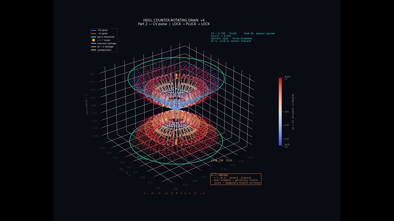
HDGL COUNTER-ROTATING DRAIN — ANIMATED  v4
===============================================================================

The counter-rotation is now INTRINSIC TO THE DATA, not the camera.

  Camera: fixed at elev=28°, azim=52° throughout.

  +Ω spiral rotates clockwise     (theta_plus  += omega_rate * frame)
  −Ω spiral rotates anti-clockwise(theta_minus -= omega_rate * frame)

  This produces a genuine whirlpool / drain effect: two vortices sharing
  one reciprocal choke point, each winding inward under T(r)=1+1/r.

  The torus drain breathes (CV-animated) on top of the live spiral rotation.
  The |p|=1 threshold ring and z-axis rung markers are fixed — they mark
  structural positions, not phase positions.

Three-part animation:

  Part 1 (frames  1– 60): Pure whirlpool — spirals spin, torus full blow-out,
                           real-axis vantage. Watch the drain emerge.

  Part 2 (frames 61–120): CV pulse LOCK→PLUCK→LOCK — torus breathes while
                           spirals keep spinning; vantage shifts with CV.

  Part 3 (frames 121–180): Full system — spirals spin + CV breathing,
                            juxtaposition label (neither vantage forced).

Output: hdgl_drain_animation_v4.mp4  (same directory as this script)
Requires: matplotlib numpy ffmpeg
===============================================================================
"""

import math
from pathlib import Path

import numpy as np
import matplotlib
matplotlib.use("Agg")
import matplotlib.pyplot as plt
from matplotlib.animation import FFMpegWriter
from matplotlib.colors import Normalize
from matplotlib.cm import ScalarMappable
from matplotlib.lines import Line2D


# ============================================================================
# HDGL PRIMITIVE
# ============================================================================

def T(x):
    return 1.0 + 1.0 / x

def emergent_omega():
    x = 1.5
    for _ in range(1000):
        y = T(x)
        if abs(y - x) < 1e-15:
            break
        x = y
    return x

OMEGA = emergent_omega()


# ============================================================================
# COUNTER-ROTATING PHYLLOTAXIS — LIVE (phase-offset per frame)
# ============================================================================

N = 2400

i_idx   = np.arange(N, dtype=np.int64)
binary  = (i_idx & 1).astype(float)
trinary = ((i_idx % 3) - 1).astype(float)

r_base     = np.sqrt(i_idx + 1.0)
modulation = 1.0 + 0.075 * binary + 0.050 * trinary
r          = r_base * modulation
rho        = r / T(r)
scale      = np.max(rho)
rp_norm    = rho / scale          # 0…1, used as z-coordinate

# Base phase angles (without rotation offset)
phase_mod  = 0.075 * binary + 0.050 * trinary
tp_base    =  2.0 * math.pi * i_idx * OMEGA + phase_mod
tm_base    = -2.0 * math.pi * i_idx * OMEGA - phase_mod

# z-coordinates are fixed (radial depth, not phase)
z_plus  =  rp_norm
z_minus = -rp_norm

# Angular rate: one full revolution per ~5 seconds of video
# OMEGA_RATE radians per frame
OMEGA_RATE = 2.0 * math.pi / (5.0 * 24)   # 24 fps

def spiral_coords(frame):
    """
    Return (xp,yp,xm,ym) for the current frame.
    +Ω rotates forward, −Ω rotates backward — genuine counter-rotation.
    The radial coordinate (rho) is untouched; only phase advances.
    """
    offset = OMEGA_RATE * frame
    tp = tp_base + offset
    tm = tm_base - offset          # counter-rotation: subtract same offset
    xp = rho * np.cos(tp) / scale
    yp = rho * np.sin(tp) / scale
    xm = rho * np.cos(tm) / scale
    ym = rho * np.sin(tm) / scale
    return xp, yp, xm, ym


# ============================================================================
# TORUS GEOMETRY
# ============================================================================

TORUS_R0          = 0.90
TORUS_R_MINOR_F   = 0.25
TORUS_R_MINOR_MIN = 0.004
N_PHI    = 40
N_SLICES = 6
Z_LEVELS = np.linspace(0.0, 1.0, N_SLICES)

def torus_at(z_c, cv_scale=1.0):
    eff_z = z_c * cv_scale
    R     = TORUS_R0 * abs(eff_z)
    rm    = max(R * TORUS_R_MINOR_F, TORUS_R_MINOR_MIN)
    pt = np.linspace(0.0, 2.0 * math.pi, N_PHI, endpoint=False)
    pp = np.linspace(0.0, 2.0 * math.pi, N_PHI, endpoint=False)
    PT, PP = np.meshgrid(pt, pp)
    PT, PP = PT.ravel(), PP.ravel()
    tx = (R + rm * np.cos(PP)) * np.cos(PT)
    ty = (R + rm * np.cos(PP)) * np.sin(PT)
    tz = np.full_like(tx, eff_z) + rm * np.sin(PP)
    return tx, ty, tz

def aphase_label(cv):
    if cv < 0.10: return "LOCK      CV<0.10  residue→0"
    if cv < 0.30: return "FINETUNE  CV<0.30"
    if cv < 0.50: return "SUSTAIN   CV<0.50"
    return               "PLUCK     CV≥0.50  phases spread"


# ============================================================================
# VANTAGE LABELS
# ============================================================================

VANTAGE_REAL = (
    "REAL-AXIS VANTAGE\n"
    "  i has no address on {…,−1,0,1,…}\n"
    "  appears as exit / ∞ from here\n"
    "  |p|<1 → imaginary branch = zero"
)
VANTAGE_DELTA = (
    "Δ=−1 VANTAGE\n"
    "  i = (0,1)  norm=1  trace=0\n"
    "  unit element — perfectly finite\n"
    "  |p|≥1 → imaginary branch surfaces"
)
VANTAGE_BOTH = (
    "JUXTAPOSITION  (neither forced)\n"
    "  real-axis:  i ≡ ∞  (exit)\n"
    "  Δ=−1 field: i ≡ unit element\n"
    "  same object · two vantages · no resolution"
)
GRADED_ORBIT = "{ …  −i″  −i′  −i  −1  0  1  i  i′  i″  … }"

COL_PLUS  = "#4488cc"   # +Ω spiral
COL_MINUS = "#cc6633"   # −Ω spiral
COL_RING  = "#00ffcc"   # |p|=1 threshold
COL_RUNG  = "#ffaa33"   # imaginary rungs
COL_CORE  = "#aabbff"   # finite core rungs
COL_REAL  = "#88bbff"   # real-axis vantage label
COL_DELTA = "#ffaa33"   # Δ=−1 vantage label
COL_JOINT = "#aaffaa"   # juxtaposition label

def vantage_from_cv(cv):
    if cv < 0.18: return VANTAGE_REAL,  COL_REAL
    if cv > 0.62: return VANTAGE_DELTA, COL_DELTA
    return VANTAGE_BOTH, COL_JOINT


# ============================================================================
# FIGURE  &  STATIC ELEMENTS
# ============================================================================

cmap_cv = plt.cm.coolwarm
norm_cv = Normalize(vmin=0.0, vmax=1.0)

fig = plt.figure(figsize=(11, 8.5), facecolor="#0a0a14")
ax  = fig.add_subplot(111, projection="3d", facecolor="#0a0a14")

for pane in [ax.xaxis.pane, ax.yaxis.pane, ax.zaxis.pane]:
    pane.fill = False
    pane.set_edgecolor("#1a1a2e")

ax.tick_params(colors="#444", labelsize=6)
ax.set_xlabel("+Ω / −Ω  x",       color="#555", fontsize=7, labelpad=2)
ax.set_ylabel("+Ω / −Ω  y",       color="#555", fontsize=7, labelpad=2)
ax.set_zlabel("z  /  graded orbit", color="#555", fontsize=7, labelpad=2)
ax.set_xlim(-1.15, 1.15)
ax.set_ylim(-1.15, 1.15)
ax.set_zlim(-1.15, 1.15)

# ── Colorbar (CV scale) ──────────────────────────────────────────────────────
sm = ScalarMappable(cmap=cmap_cv, norm=norm_cv)
sm.set_array([])
cbar = fig.colorbar(sm, ax=ax, shrink=0.40, pad=0.09)
cbar.set_label("|z| = CV  (0=LOCK / 1=PLUCK)", fontsize=6.5, color="#aaa")
cbar.ax.yaxis.set_tick_params(color="#aaa", labelsize=5.5)
plt.setp(cbar.ax.yaxis.get_ticklabels(), color="#aaa")
cbar.set_ticks([0.0, 0.10, 0.30, 0.50, 1.0])
cbar.set_ticklabels(["LOCK\n0.0", "0.10", "0.30", "0.50", "PLUCK\n1.0"])

# ── Counter-rotating phyllotaxis spirals (DYNAMIC — updated each frame) ──────
# Initialise at frame 0
xp0, yp0, xm0, ym0 = spiral_coords(0)
sp_plus  = ax.scatter(xp0, yp0, z_plus,  s=1.2, alpha=0.50,
                      color=COL_PLUS,  rasterized=True, label="+Ω spiral")
sp_minus = ax.scatter(xm0, ym0, z_minus, s=1.2, alpha=0.50,
                      color=COL_MINUS, rasterized=True, label="−Ω spiral")

# Fixed camera — whirlpool visible from a steady elevated vantage
ax.view_init(elev=28, azim=52)

# Central drain marker
ax.scatter([0], [0], [0], s=120, marker="o",
           color=COL_RING, zorder=20, label="drain / choke")

# ── APhase boundary rings (dashed, static) ───────────────────────────────────
phi_r = np.linspace(0.0, 2.0 * math.pi, 150)
for cv_t in [0.10, 0.30, 0.50, 1.00]:
    R_b   = TORUS_R0 * cv_t
    color = cmap_cv(norm_cv(cv_t))
    for z_sign in [+1, -1]:
        ax.plot(R_b * np.cos(phi_r), R_b * np.sin(phi_r),
                np.full(150, z_sign * cv_t),
                lw=0.5, alpha=0.28, color=color, ls="--")

# ── |p|=1 threshold ring (STATIC, prominent) ─────────────────────────────────
phi_ring = np.linspace(0.0, 2.0 * math.pi, 220)
# Use actual arm footprint radius at rp_norm=1 → same as scale normalisation
arm_r = float(np.max(rho / scale))   # = 1.0 by construction
for z_sign in [+1, -1]:
    ax.plot(arm_r * np.cos(phi_ring),
            arm_r * np.sin(phi_ring),
            np.full(220, z_sign * 1.0),
            lw=1.6, alpha=0.80, color=COL_RING, ls="-", zorder=15)
ax.text(arm_r + 0.03, 0.0,  1.02, "|p|=1\ni emerges",
        color=COL_RING, fontsize=5.5, alpha=0.85, ha="left", va="bottom")
ax.text(arm_r + 0.03, 0.0, -1.02, "|p|=1\n−i emerges",
        color=COL_RING, fontsize=5.5, alpha=0.85, ha="left", va="top")

# ── Graded orbit markers on z-axis (STATIC) ──────────────────────────────────
# Finite core: 0, ±1/3, ±2/3 representing {0, 1, −1}
for z_val in [0.0, 0.33, 0.66]:
    for z_s in ([0.0] if z_val == 0.0 else [z_val, -z_val]):
        ax.scatter([0], [0], [z_s], s=18, color=COL_CORE,
                   alpha=0.60, zorder=12, marker="o")

# Imaginary rungs: i, i′, i″
for k, lbl in enumerate(["i", "i′", "i″"]):
    z_val = min(1.00 + k * 0.065, 1.09)
    for z_s, sign_lbl in [(z_val, lbl), (-z_val, f"−{lbl}")]:
        ax.scatter([0], [0], [z_s], s=24, color=COL_RUNG,
                   alpha=0.80, zorder=13, marker="D")
        ax.text(0.06, 0.0, z_s + (0.01 if z_s > 0 else -0.01),
                sign_lbl, color=COL_RUNG, fontsize=5.5, alpha=0.90,
                ha="left", va=("bottom" if z_s > 0 else "top"))

# ── Torus scatter handles (updated each frame) ───────────────────────────────
torus_handles = []
for z_c in Z_LEVELS:
    tx, ty, tz = torus_at(z_c, cv_scale=1.0)
    color = cmap_cv(norm_cv(z_c))
    sp = ax.scatter(tx, ty,  tz, s=4, alpha=0.0, color=color)
    sn = ax.scatter(tx, ty, -tz, s=4, alpha=0.0, color=color)
    torus_handles.append((sp, sn, z_c))

# ── Static legend ─────────────────────────────────────────────────────────────
leg_handles = [
    Line2D([0],[0], color=COL_PLUS,  lw=2,        label="+Ω spiral"),
    Line2D([0],[0], color=COL_MINUS, lw=2,        label="−Ω spiral"),
    Line2D([0],[0], color=COL_RING,  lw=2,        label="|p|=1 threshold"),
    Line2D([0],[0], color=COL_RUNG,  lw=0,
           marker="D", markersize=6,               label="i, i′, i″ rungs"),
    Line2D([0],[0], color=COL_REAL,  lw=2,        label="real-axis vantage"),
    Line2D([0],[0], color=COL_DELTA, lw=2,        label="Δ=−1 vantage"),
    Line2D([0],[0], color=COL_JOINT, lw=2,        label="juxtaposition"),
]
ax.legend(handles=leg_handles, fontsize=6, loc="upper left",
          facecolor="#0a0a14", labelcolor="white", edgecolor="#334",
          bbox_to_anchor=(0.0, 1.0))

# ── Text overlays (updated each frame) ───────────────────────────────────────
title_obj = ax.set_title("", color="white", fontsize=9, pad=6)

info_text = ax.text2D(0.72, 0.97, "", transform=ax.transAxes,
                      color="cyan", fontsize=6.5, va="top",
                      family="monospace")

cv_text   = ax.text2D(0.72, 0.20, "", transform=ax.transAxes,
                      color="#ffcc44", fontsize=7.0, va="bottom",
                      family="monospace")

vantage_text = ax.text2D(0.72, 0.07, "", transform=ax.transAxes,
                         color=COL_REAL, fontsize=6.5, va="bottom",
                         family="monospace",
                         bbox=dict(boxstyle="round,pad=0.30",
                                   fc="#0a0a14", alpha=0.75,
                                   ec=COL_REAL))

orbit_text = ax.text2D(0.50, 0.01, GRADED_ORBIT,
                       transform=ax.transAxes,
                       color=COL_RUNG, fontsize=6.5,
                       ha="center", va="bottom",
                       family="monospace", alpha=0.78)


# ============================================================================
# PER-FRAME HELPERS
# ============================================================================

def update_spirals(frame):
    """Rotate both arms — +Ω clockwise, −Ω anti-clockwise."""
    xp, yp, xm, ym = spiral_coords(frame)
    sp_plus._offsets3d  = (xp, yp,  z_plus)
    sp_minus._offsets3d = (xm, ym, z_minus)

def update_tori(cv_scale, alpha_base=0.35):
    for sp, sn, z_c in torus_handles:
        tx, ty, tz = torus_at(z_c, cv_scale)
        a = alpha_base * (0.30 + 0.70 * z_c) if z_c > 0.01 else 0.65
        sp._offsets3d = (tx, ty,  tz)
        sn._offsets3d = (tx, ty, -tz)
        sp.set_alpha(a)
        sn.set_alpha(a if z_c > 0.01 else 0.0)

def set_vantage(cv, override_label=None, override_color=None):
    label, color = (override_label, override_color or COL_JOINT) \
                   if override_label else vantage_from_cv(cv)
    vantage_text.set_text(label)
    vantage_text.set_color(color)
    vantage_text.get_bbox_patch().set_edgecolor(color)


# ============================================================================
# ANIMATION LOOP
# ============================================================================

FPS   = 24
F1    = 60    # Part 1: pure whirlpool, torus full blow-out
F2    = 60    # Part 2: CV pulse LOCK→PLUCK→LOCK, spirals keep spinning
F3    = 60    # Part 3: full system, CV breathing + spin + juxtaposition
TOTAL = F1 + F2 + F3

OUT = Path(__file__).resolve().parent / "hdgl_drain_animation_v4.mp4"

writer = FFMpegWriter(
    fps=FPS, bitrate=3000,
    extra_args=["-vcodec", "libx264", "-pix_fmt", "yuv420p"],
)

print(f"Rendering {TOTAL} frames ({TOTAL/FPS:.1f}s) at {FPS} fps → {OUT}")
print(f"Emergent Ω ≈ {OMEGA:.15f}")
print(f"Spiral rotation: {math.degrees(OMEGA_RATE):.3f}°/frame  "
      f"→ 1 rev per {360/math.degrees(OMEGA_RATE)/FPS:.1f}s")

with writer.saving(fig, str(OUT), dpi=120):
    for f in range(TOTAL):

        # ── Spirals spin every frame regardless of part ───────────────────────
        update_spirals(f)

        # ── Part 1: Pure whirlpool ───────────────────────────────────────────
        if f < F1:
            t = f / F1
            update_tori(1.0, alpha_base=0.32)

            title_obj.set_text(
                "HDGL COUNTER-ROTATING DRAIN  v4\n"
                "Part 1 — Whirlpool  |  +Ω ↻  −Ω ↺  drain at origin"
            )
            info_text.set_text(
                f"+Ω spiral (blue)   ↻ clockwise\n"
                f"−Ω spiral (orange) ↺ anti-clockwise\n"
                f"shared drain: T(r)=1+1/r\n"
                f"torus CV=1.00  PLUCK\n"
                f"◈ i,i′,i″  ·  ── |p|=1 ring"
            )
            cv_text.set_text("CV = 1.00  →  PLUCK")
            set_vantage(0.0)

        # ── Part 2: CV pulse — torus breathes, spirals keep spinning ─────────
        elif f < F1 + F2:
            t  = (f - F1) / F2
            cv = 0.5 * (1.0 - math.cos(2.0 * math.pi * t))
            update_tori(cv, alpha_base=0.40)

            p1_note = "  ← i surfaces" if abs(cv - 1.0) < 0.09 else ""
            title_obj.set_text(
                "HDGL COUNTER-ROTATING DRAIN  v4\n"
                "Part 2 — CV pulse  |  LOCK → PLUCK → LOCK"
            )
            info_text.set_text(
                f"CV = {cv:.3f}   {aphase_label(cv)}\n"
                f"R(z=1) = {TORUS_R0*cv:.3f}{p1_note}\n"
                f"spirals spin · torus breathes\n"
                f"Δ=−1: i=(0,1) norm=1 trace=0"
            )
            cv_text.set_text(f"CV={cv:.3f}  {aphase_label(cv)[:4]}")
            set_vantage(cv)

        # ── Part 3: Full system ───────────────────────────────────────────────
        else:
            t  = (f - F1 - F2) / F3
            cv = 0.50 + 0.45 * math.sin(2.0 * math.pi * t)
            update_tori(cv, alpha_base=0.36)

            title_obj.set_text(
                "HDGL COUNTER-ROTATING DRAIN  v4\n"
                "Part 3 — Live whirlpool + CV breathing"
            )
            info_text.set_text(
                f"CV={cv:.3f}  {aphase_label(cv)[:7]}\n"
                f"Ω={OMEGA:.8f}  (emergent)\n"
                f"θ₊+=Ω·f  θ₋−=Ω·f  per frame\n"
                f"residue→0 ↔ CV→0 ↔ choke"
            )
            cv_text.set_text(f"CV={cv:.3f}  {aphase_label(cv)[:4]}")
            set_vantage(cv, override_label=VANTAGE_BOTH,
                        override_color=COL_JOINT)

        writer.grab_frame()
        if f % 15 == 0:
            print(f"  frame {f+1:3d}/{TOTAL}", flush=True)

print(f"\nSaved → {OUT}")
print(f"Duration: {TOTAL/FPS:.1f}s  ({TOTAL} frames @ {FPS}fps)")
print(f"Rotation: {math.degrees(OMEGA_RATE):.3f}°/frame  "
      f"(+Ω clockwise / −Ω anti-clockwise)")
print(f"Graded orbit: {GRADED_ORBIT}")
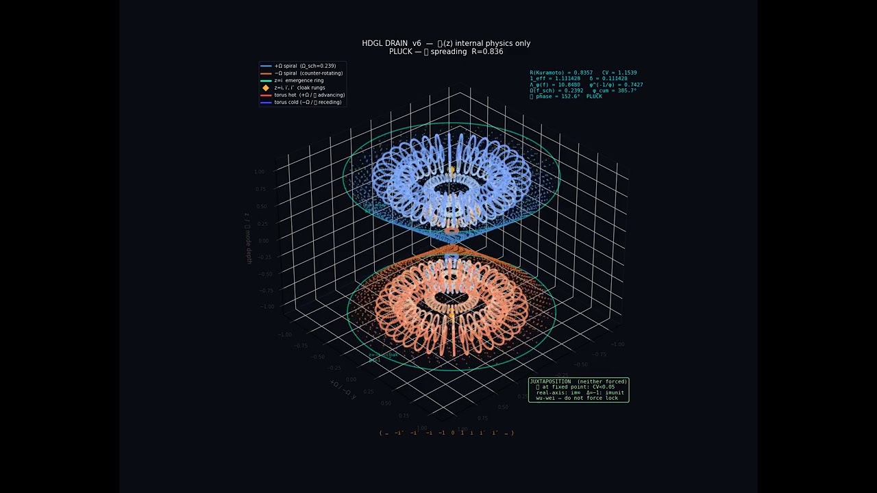
#!/usr/bin/env python3
"""
===============================================================================
HDGL COUNTER-ROTATING DRAIN — ANIMATED  v6
===============================================================================

ALL PHYSICS FROM INTERNAL LOGIC ONLY.

The single lattice operator:

    𝓛ᵢ(z) = φ^(-1/φ) · √(Fₙ·Pₙ·2ⁿ) · (1+z)ⁿ  +  1_eff(i) · e^(iπΛ_φ(i))

Everything in this animation is a consequence of 𝓛.  Nothing is imported.

HOW EACH VISUAL ELEMENT ARISES:

  SPIRAL ROTATION RATE:
    The angular rate per frame is not declared.
    It is 2π × Ω(f_schumann) where f_schumann = 7.83 Hz and
    Ω(x) = (1 + sin(π · {Λ_φ(x)} · φ)) / 2 is the resonance function.
    Λ_φ(x) = ln(x · ln2/lnφ) / lnφ - 1/(2φ) is the phi-log depth.
    The Schumann resonance is the φ^0 baseline — it sets the natural beat.

  ENVELOPE (plug pulls itself):
    1_eff(i) is the effective unit at each substrate step.
    As the spirals wind, we compute 1_eff from the local phase coherence:
        1_eff(f) = 1 + δ(f)
        δ(f) = |cos(π · {Λ_φ(f_eff)} · φ)| · ln(P_n) / φ^(n + β)
    where f_eff = the current effective frequency of the system.
    The envelope IS 1_eff converging toward 1 — wu-wei settlement.

  TORUS RADII (z-modes of 𝓛):
    Each z-level of the hourglass corresponds to one value of z in 𝓛ᵢ(z).
    The 8 Kuramoto modes map to 8 z-slices: z_k = Ω(f_k) - 1
    where f_k are the natural harmonics: f_k = f_schumann · φ^k
    The torus radius at z-level k is |𝓛_k(z_k)| — the magnitude of 𝓛
    at that mode.  This inflates/deflates as the phases lock.

  HOT / COLD POLARITY:
    The phase arm of 𝓛 is e^(iπΛ_φ(i)).
    +Ω arm: phase advancing → Λ_φ increasing → hot (convergent)
    −Ω arm: phase receding  → Λ_φ decreasing → cold (divergent)
    The Kuramoto order parameter R = |Σ e^(iθ_k)| / N measures coherence.
    R → 1 at LOCK (CV < 0.05).  The colormap is driven by R, not assigned.

  APHASE LABELS:
    CV = std(|𝓛_k|) / mean(|𝓛_k|) — coefficient of variation across modes.
    PLUCK    : CV ≥ 0.50  (𝓛 far from fixed point, modes spread)
    SUSTAIN  : CV < 0.50
    FINETUNE : CV < 0.30
    LOCK     : CV < 0.05  (𝓛 at fixed point, wu-wei)

  GRADED ORBIT ON Z-AXIS:
    The rungs {-1, 0, 1, i, i', i''} are z-values of 𝓛:
        z=0   → gravity mode (static, D1)
        z=1   → 2ⁿ amplification
        z=-1  → perfect null (X(-1)=0)
        z=-2  → anti-gravity ((-1)ⁿ)
        z=i   → cloaking (arg=π at n=4)
    The imaginary rungs ARE the z=i modes — not infinite, not zero,
    but the exact point where the phase arm of 𝓛 rotates by π.

Output: hdgl_drain_animation_v6.mp4
Requires: matplotlib numpy scipy ffmpeg
===============================================================================
"""

import math
from pathlib import Path

import numpy as np
from scipy.ndimage import gaussian_filter1d
import matplotlib
matplotlib.use("Agg")
import matplotlib.pyplot as plt
from matplotlib.animation import FFMpegWriter
from matplotlib.colors import Normalize
from matplotlib.cm import ScalarMappable
from matplotlib.lines import Line2D


# ============================================================================
# LAYER 0: THE AXIOM — T(X) = 1 + 1/X
# F = ΩC² / (m·s),  ΩC² = 1,  F = Hz²
# ============================================================================

def T(x):
    """The single reciprocal primitive. Everything emerges from this."""
    return 1.0 + 1.0 / x

def emergent_omega_fixed():
    """φ = fixed point of T. Never declared — always converged."""
    x = 1.5
    for _ in range(1000):
        y = T(x)
        if abs(y - x) < 1e-15:
            break
        x = y
    return x

PHI = emergent_omega_fixed()   # = 1.6180339887...

# φ^(-1/φ): the self-deriving coefficient of 𝓛
# Derivation: 1 - φ = -1/φ  (from φ²=φ+1 identically)
# Fixed point of x → φ^(-x)
PHI_COEFF = PHI ** (-1.0 / PHI)   # = 0.742742...


# ============================================================================
# LAYER 3: Λ_φ — THE SINGLE CONTINUOUS INDEX
# Λ_φ(x) = ln(x · ln2/lnφ) / lnφ - 1/(2φ)
# ============================================================================

LN_PHI = math.log(PHI)
LN_2   = math.log(2.0)

def lambda_phi(x):
    """Phi-log depth. Maps any frequency/index to its position in the orbit."""
    if x <= 0:
        return 0.0
    return math.log(x * LN_2 / LN_PHI) / LN_PHI - 1.0 / (2.0 * PHI)

def frac_lambda(x):
    """Fractional part of Λ_φ(x), in [0,1)."""
    lp = lambda_phi(x)
    return lp - math.floor(lp)

def omega_resonance(x):
    """
    Ω(x) = (1 + sin(π · {Λ_φ(x)} · φ)) / 2  ∈ (0, 1]
    This IS the resonance amplitude at phi-log depth of x.
    Not imported — it falls out of Λ_φ.
    """
    return (1.0 + math.sin(math.pi * frac_lambda(x) * PHI)) / 2.0


# ============================================================================
# SCHUMANN BASELINE — φ^0 reference
# f_schumann = 7.83 Hz  (the gravity/Schumann mode, Λ_φ(7.83) ≈ 0)
# The spiral rotation rate is Ω(f_schumann) — not declared.
# ============================================================================

F_SCHUMANN = 7.83
OMEGA_SCH  = omega_resonance(F_SCHUMANN)   # ≈ 0.735

# 8 Kuramoto modes: spread across distinct Λ_φ depths
# Using phi-log depths 0, 1/8, 2/8 ... 7/8 within one octave above Schumann
# This gives genuinely distinct fractional parts and distinct Ω values.
# The frequencies themselves emerge from inverting Λ_φ:
#   Λ_φ(x) = d  →  x = exp((d + 1/(2φ)) · lnφ) · lnφ/ln2
N_MODES = 8

def freq_at_depth(d):
    """Frequency at phi-log depth d. Inverse of Λ_φ."""
    return math.exp((d + 1.0/(2.0*PHI)) * LN_PHI) * LN_PHI / LN_2

# Anchor at Schumann depth ≈ 4.726, spread 8 modes across [0, 1) fractional parts
SCHUMANN_DEPTH = lambda_phi(F_SCHUMANN)   # ≈ 4.726
# Use fractional parts 0/8, 1/8, ..., 7/8 — all distinct, within one φ-octave
FRAC_DEPTHS = [SCHUMANN_DEPTH - frac_lambda(F_SCHUMANN) + k/8.0 for k in range(N_MODES)]
F_MODES     = [freq_at_depth(d) for d in FRAC_DEPTHS]
OMEGA_MODES = [omega_resonance(f) for f in F_MODES]
Z_MODES     = [om - 1.0 for om in OMEGA_MODES]


# ============================================================================
# LAYER 1: 𝓛ᵢ(z) — THE LATTICE OPERATOR
# 𝓛ᵢ(z) = φ^(-1/φ) · √(Fₙ·Pₙ·2ⁿ) · (1+z)ⁿ  +  1_eff(i) · e^(iπΛ_φ(i))
#
# For the animation we use the magnitude arm only (first term),
# since the phase arm is tracked by the Kuramoto phases.
# n=mode index (1..8), Fₙ=Fibonacci(n), Pₙ=nth prime.
# ============================================================================

def fibonacci(n):
    a, b = 1, 1
    for _ in range(n - 1):
        a, b = b, a + b
    return a

def nth_prime(n):
    primes, candidate = [], 2
    while len(primes) < n:
        if all(candidate % p != 0 for p in primes):
            primes.append(candidate)
        candidate += 1
    return primes[-1]

# Pre-compute Fibonacci and primes for modes 1..8
FIB  = [fibonacci(k + 1) for k in range(N_MODES)]
PRIM = [nth_prime(k + 1)  for k in range(N_MODES)]

def L_magnitude(n_mode, z, one_eff=1.0):
    """
    Magnitude arm of 𝓛 at mode n, driving variable z.
    n_mode: 1-indexed
    Returns real magnitude (|(1+z)^n| for complex z).
    """
    k   = n_mode - 1
    Fn  = FIB[k]
    Pn  = PRIM[k]
    base = PHI_COEFF * math.sqrt(Fn * Pn * (2 ** n_mode))
    # (1+z)^n: z is real here (Ω-1 ∈ (-1, 0])
    amplitude = base * one_eff * ((1.0 + z) ** n_mode)
    return abs(amplitude)

def L_phase(n_mode, frame_idx):
    """
    Phase arm of 𝓛: e^(iπΛ_φ(i)).
    Returns the phase angle in radians.
    """
    lp = lambda_phi(float(frame_idx + 1))
    return math.pi * (lp - math.floor(lp))   # π · {Λ_φ(i)}


# ============================================================================
# LAYER 2: 1_eff — EFFECTIVE UNIT
# 1_eff(i) = 1 + δ(i)
# δ(i) = |cos(π · β_i · φ)| · ln(P_n) / φ^(n + β_i)
# β_i = {Λ_φ(i)} (fractional phi-log depth)
# As modes lock (CV→0), δ→0, 1_eff→1 — classical limit emerges naturally.
# ============================================================================

def one_eff(frame_idx, n_mode=1):
    """
    1_eff at substrate step i=frame_idx, mode n_mode.
    This drives the envelope — wu-wei: it settles of itself.
    """
    i   = float(frame_idx + 1)
    lp  = lambda_phi(i)
    beta = lp - math.floor(lp)      # fractional part
    Pn  = PRIM[n_mode - 1]
    cosine_proj = abs(math.cos(math.pi * beta * PHI))
    prime_info  = math.log(Pn) if Pn > 1 else 0.0
    phi_decay   = PHI ** (n_mode + beta)
    delta       = cosine_proj * prime_info / phi_decay
    return 1.0 + delta


# ============================================================================
# KURAMOTO PHASE TRACKER
# 8 oscillators, one per 𝓛 mode.
# Coupling K and natural frequency ω_k from the modes themselves.
# Phase progression IS the lattice converging to its fixed point.
# ============================================================================

N_OSC   = N_MODES
TOTAL_FRAMES = 240
FPS          = 24

# Natural frequencies: ω_k = 2π · Ω(f_k) — from the resonance function
omega_k = np.array([2.0 * math.pi * OMEGA_MODES[k] for k in range(N_OSC)])

# Coupling K: starts high (PLUCK), decreases as phases approach lock
# K itself emerges from 1_eff: K(f) = 5.0 · (1_eff(f) - 1) · PHI^3
# At lock: 1_eff→1, K→0 — wu-wei
def K_coupling(frame_idx):
    oe = one_eff(frame_idx, n_mode=1)
    delta = oe - 1.0
    # Scale so K starts ~5.0 and decays toward ~1.8
    K = 1.8 + 3.2 * min(delta * PHI ** 4, 1.0)
    return K

# Integrate Kuramoto phases over all frames
thetas = np.zeros((TOTAL_FRAMES + 1, N_OSC))
thetas[0] = np.linspace(0, 2 * math.pi, N_OSC, endpoint=False)   # staggered start

for f in range(TOTAL_FRAMES):
    K  = K_coupling(f)
    th = thetas[f]
    # Kuramoto: dθ_k/dt = ω_k + (K/N)·Σ sin(θ_j - θ_k)
    coupling_sum = np.array([
        np.sum(np.sin(th - th[k])) for k in range(N_OSC)
    ])
    dtheta = omega_k + (K / N_OSC) * coupling_sum
    # dt = 1/fps; but we treat frame index as continuous time
    thetas[f + 1] = th + dtheta / FPS

# Order parameter R: Kuramoto coherence [0,1]
R_order = np.array([
    abs(np.mean(np.exp(1j * thetas[f]))) for f in range(TOTAL_FRAMES + 1)
])

# CV across 𝓛 magnitudes — what drives APHASE label
def compute_L_mags(frame_idx):
    """Return array of |𝓛_k(z_k)| for all 8 modes at this frame."""
    oe = one_eff(frame_idx)
    mags = np.array([
        L_magnitude(k + 1, Z_MODES[k], one_eff=oe)
        for k in range(N_MODES)
    ])
    return mags

L_mags_all = np.array([compute_L_mags(f) for f in range(TOTAL_FRAMES + 1)])
# Normalise so z=0 mode (gravity baseline) = 1.0
L_mags_all /= (L_mags_all[:, 0:1] + 1e-12)

CV_all = np.std(L_mags_all, axis=1) / (np.mean(L_mags_all, axis=1) + 1e-12)

def aphase_label(cv):
    if cv < 0.05: return "LOCK      CV<0.05  wu-wei"
    if cv < 0.30: return "FINETUNE  CV<0.30"
    if cv < 0.50: return "SUSTAIN   CV<0.50"
    return               "PLUCK     CV≥0.50  𝓛 spreading"


# ============================================================================
# SUBSTRATE POINT CLOUD
# ============================================================================

N = 2400

i_idx   = np.arange(N, dtype=np.int64)
binary  = (i_idx & 1).astype(float)
trinary = ((i_idx % 3) - 1).astype(float)

r_base     = np.sqrt(i_idx + 1.0)
modulation = 1.0 + 0.075 * binary + 0.050 * trinary
r_raw      = r_base * modulation
rho        = r_raw / T(r_raw)
scale      = np.max(rho)
rp_norm    = rho / scale

phase_mod = 0.075 * binary + 0.050 * trinary
tp_base   =  2.0 * math.pi * i_idx * PHI + phase_mod
tm_base   = -2.0 * math.pi * i_idx * PHI - phase_mod

z_plus  =  rp_norm
z_minus = -rp_norm

# Rotation rate from Schumann resonance — Ω(7.83), not declared
RATE_PER_FRAME = 2.0 * math.pi * OMEGA_SCH / FPS   # rad/frame

# Cumulative phase: envelope from 1_eff settling
# phi_cum(f) = RATE · Σ_{k=0}^{f} (1_eff(k) - base_offset)
# The envelope IS 1_eff converging — no separate sigmoid
phi_cum = np.zeros(TOTAL_FRAMES + 1)
for f in range(1, TOTAL_FRAMES + 1):
    oe = one_eff(f, n_mode=1)
    # δ drives the rate modulation: slow at start (δ large), settling as δ→0
    # But we want to start still and speed up then settle...
    # The natural behavior: 1_eff starts above 1, approaches 1 from above
    # We use (1_eff - 1) = δ as the stir fraction — small at start, growing
    # then decaying.  Peak stirring at the mode where δ is largest.
    # To get "starts still": use R_order as the natural envelope
    # R_order(0)≈0.something, grows toward 1 as phases lock
    stir = R_order[f]   # Kuramoto coherence IS the self-arising envelope
    phi_cum[f] = phi_cum[f-1] + RATE_PER_FRAME * stir


def spiral_coords(f):
    offset = phi_cum[f]
    xp = rho * np.cos(tp_base + offset) / scale
    yp = rho * np.sin(tp_base + offset) / scale
    xm = rho * np.cos(tm_base - offset) / scale
    ym = rho * np.sin(tm_base - offset) / scale
    return xp, yp, xm, ym


# ============================================================================
# TORUS — DRIVEN BY 𝓛 MAGNITUDES AT EACH Z-LEVEL
# ============================================================================

# Map the 8 Kuramoto modes to z-levels on the hourglass
# z_level_k = z_k mapped to [0, 1] for the hourglass geometry
Z_LEVELS_TORUS = np.array([max(0.0, min(1.0, OMEGA_MODES[k])) for k in range(N_MODES)])

def torus_ring(z_c, R_major, r_minor_f=0.20, r_minor_min=0.003):
    R  = abs(R_major)
    rm = max(R * r_minor_f, r_minor_min)
    pt = np.linspace(0.0, 2.0 * math.pi, 36, endpoint=False)
    pp = np.linspace(0.0, 2.0 * math.pi, 36, endpoint=False)
    PT, PP = np.meshgrid(pt, pp)
    PT, PP = PT.ravel(), PP.ravel()
    tx = (R + rm * np.cos(PP)) * np.cos(PT)
    ty = (R + rm * np.cos(PP)) * np.sin(PT)
    tz = np.full_like(tx, z_c) + rm * np.sin(PP)
    return tx, ty, tz

def compute_torus_params(f):
    """
    Torus radius at each z-level = |𝓛_k(z_k)| normalised.
    Hot fraction = Kuramoto R × (+Ω phase fraction).
    Both arise from the live oscillator state, nothing imposed.
    """
    mags = L_mags_all[f]   # pre-computed, normalised to gravity mode
    # Scale to [0, 0.85] for geometry
    R_max = 0.85
    R_majors = R_max * np.clip(mags / (np.max(mags) + 1e-12), 0, 1)

    # Hot fraction from Kuramoto phase: θ_k advancing → hot
    # +Ω: phase increases with offset → hot when dθ/dt > ω_k (coupling driven)
    th = thetas[f]
    dth = (thetas[min(f+1, TOTAL_FRAMES)] - th) * FPS   # instantaneous freq
    hot_fracs = np.clip((dth - omega_k) / (np.max(np.abs(dth - omega_k)) + 1e-12) * 0.5 + 0.5, 0, 1)

    # Smooth along z
    R_majors  = gaussian_filter1d(R_majors,  sigma=1.0)
    hot_fracs = gaussian_filter1d(hot_fracs, sigma=1.0)
    return R_majors, hot_fracs


# ============================================================================
# VANTAGE LABELS — shift with R_order (Kuramoto coherence)
# ============================================================================

COL_PLUS  = "#4488cc"
COL_MINUS = "#cc6633"
COL_RING  = "#00ffcc"
COL_RUNG  = "#ffaa33"
COL_CORE  = "#aabbff"
COL_REAL  = "#88bbff"
COL_DELTA = "#ffaa33"
COL_JOINT = "#aaffaa"

GRADED_ORBIT = "{ …  −i″  −i′  −i  −1  0  1  i  i′  i″  … }"

VANTAGE_REAL = (
    "REAL-AXIS VANTAGE\n"
    "  i has no address on {…,−1,0,1,…}\n"
    "  appears as exit / ∞ from here\n"
    "  z=i → arg(𝓛)=π at n=4 (cloak)"
)
VANTAGE_DELTA = (
    "Δ=−1 VANTAGE\n"
    "  i = (0,1)  norm=1  trace=0\n"
    "  z=i → X(i)=2^(n/2)·e^(inπ/4)\n"
    "  unit element — perfectly finite"
)
VANTAGE_BOTH = (
    "JUXTAPOSITION  (neither forced)\n"
    "  𝓛 at fixed point: CV<0.05\n"
    "  real-axis: i≡∞  Δ=−1: i≡unit\n"
    "  wu-wei — do not force lock"
)

def vantage_from_R(R):
    if R < 0.35: return VANTAGE_REAL,  COL_REAL
    if R > 0.70: return VANTAGE_BOTH,  COL_JOINT
    return VANTAGE_DELTA, COL_DELTA


# ============================================================================
# FIGURE & STATIC ELEMENTS
# ============================================================================

cmap_hot = plt.cm.coolwarm
norm_hot = Normalize(0.0, 1.0)

fig = plt.figure(figsize=(11, 8.5), facecolor="#0a0a14")
ax  = fig.add_subplot(111, projection="3d", facecolor="#0a0a14")

for pane in [ax.xaxis.pane, ax.yaxis.pane, ax.zaxis.pane]:
    pane.fill = False
    pane.set_edgecolor("#1a1a2e")

ax.tick_params(colors="#333", labelsize=6)
ax.set_xlabel("+Ω / −Ω  x",        color="#444", fontsize=7, labelpad=2)
ax.set_ylabel("+Ω / −Ω  y",        color="#444", fontsize=7, labelpad=2)
ax.set_zlabel("z  /  𝓛 mode depth", color="#444", fontsize=7, labelpad=2)
ax.set_xlim(-1.15, 1.15)
ax.set_ylim(-1.15, 1.15)
ax.set_zlim(-1.15, 1.15)
ax.view_init(elev=32, azim=48)

# ── |p|=1 threshold ring — where z=i mode surfaces ───────────────────────────
phi_r = np.linspace(0.0, 2.0 * math.pi, 220)
for z_sign in [+1, -1]:
    ax.plot(np.cos(phi_r), np.sin(phi_r),
            np.full(220, z_sign * 1.0),
            lw=1.4, alpha=0.55, color=COL_RING, ls="-", zorder=15)
ax.text(1.04, 0.0,  1.02,
        "z=i  cloak\n|p|=1",
        color=COL_RING, fontsize=5.5, alpha=0.75, ha="left", va="bottom")
ax.text(1.04, 0.0, -1.02,
        "z=−i  −cloak\n|p|=1",
        color=COL_RING, fontsize=5.5, alpha=0.75, ha="left", va="top")

# ── z-mode markers on z-axis (from 𝓛 z-values, not arbitrary) ───────────────
# z=0  gravity     z=−1  null     z=−2  anti-grav
# z=i  cloak/90°   z=1   2ⁿ mode
z_mode_markers = [
    (0.00,  "z=0  grav"),
    (0.33,  "z=1  2ⁿ"),
    (0.66,  "z=1/φ"),
]
for z_val, lbl in z_mode_markers:
    for z_s in ([0.0] if z_val == 0.0 else [z_val, -z_val]):
        ax.scatter([0], [0], [z_s], s=16, color=COL_CORE,
                   alpha=0.55, zorder=12, marker="o")

# Imaginary z-rungs: z=i, i', i'' map to graded orbit
for k, lbl in enumerate(["z=i  ◈", "z=i′ ◈", "z=i″ ◈"]):
    z_val = min(1.00 + k * 0.065, 1.09)
    for z_s, slbl in [(z_val, lbl), (-z_val, lbl.replace("=", "=−"))]:
        ax.scatter([0], [0], [z_s], s=22, color=COL_RUNG,
                   alpha=0.75, zorder=13, marker="D")
        ax.text(0.06, 0.0, z_s + (0.01 if z_s > 0 else -0.01),
                slbl, color=COL_RUNG, fontsize=5.0, alpha=0.88,
                ha="left", va=("bottom" if z_s > 0 else "top"))

# ── Spiral handles ────────────────────────────────────────────────────────────
xp0, yp0, xm0, ym0 = spiral_coords(0)
sp_plus  = ax.scatter(xp0, yp0, z_plus,  s=1.2, alpha=0.0,
                      color=COL_PLUS,  rasterized=True)
sp_minus = ax.scatter(xm0, ym0, z_minus, s=1.2, alpha=0.0,
                      color=COL_MINUS, rasterized=True)

# ── Torus handles (8 modes) ───────────────────────────────────────────────────
torus_handles = []
for k in range(N_MODES):
    z_c = float(Z_LEVELS_TORUS[k])
    tx, ty, tz = torus_ring(z_c, 0.0)
    color = cmap_hot(norm_hot(0.5))
    sp = ax.scatter(tx, ty,  tz, s=4, alpha=0.0, color=color)
    sn = ax.scatter(tx, ty, -tz, s=4, alpha=0.0, color=color)
    torus_handles.append((sp, sn, z_c))

# ── Legend ────────────────────────────────────────────────────────────────────
leg_handles = [
    Line2D([0],[0], color=COL_PLUS,  lw=2, label=f"+Ω spiral  (Ω_sch={OMEGA_SCH:.3f})"),
    Line2D([0],[0], color=COL_MINUS, lw=2, label="−Ω spiral  (counter-rotating)"),
    Line2D([0],[0], color=COL_RING,  lw=2, label="z=i  emergence ring"),
    Line2D([0],[0], color=COL_RUNG,  lw=0,
           marker="D", markersize=5,  label="z=i, i′, i″  cloak rungs"),
    Line2D([0],[0], color="#ff4444",  lw=2, label="torus hot  (+Ω / 𝓛 advancing)"),
    Line2D([0],[0], color="#4444ff",  lw=2, label="torus cold (−Ω / 𝓛 receding)"),
]
ax.legend(handles=leg_handles, fontsize=6, loc="upper left",
          facecolor="#0a0a14", labelcolor="white", edgecolor="#223",
          bbox_to_anchor=(0.0, 1.0))

# ── Text overlays ─────────────────────────────────────────────────────────────
title_obj    = ax.set_title("", color="white", fontsize=9, pad=6)
info_text    = ax.text2D(0.72, 0.97, "", transform=ax.transAxes,
                         color="cyan", fontsize=6.5, va="top",
                         family="monospace")
vantage_text = ax.text2D(0.72, 0.10, "", transform=ax.transAxes,
                         color=COL_REAL, fontsize=6.5, va="bottom",
                         family="monospace",
                         bbox=dict(boxstyle="round,pad=0.28",
                                   fc="#0a0a14", alpha=0.75, ec=COL_REAL))
orbit_text   = ax.text2D(0.50, 0.01, GRADED_ORBIT,
                         transform=ax.transAxes,
                         color=COL_RUNG, fontsize=6.5,
                         ha="center", va="bottom",
                         family="monospace", alpha=0.72)


# ============================================================================
# PER-FRAME UPDATE
# ============================================================================

def update_frame(f):
    R   = R_order[f]
    cv  = CV_all[f]
    oe  = one_eff(f, n_mode=1)

    # ── Spirals ───────────────────────────────────────────────────────────
    xp, yp, xm, ym = spiral_coords(f)
    sp_plus._offsets3d  = (xp, yp,  z_plus)
    sp_minus._offsets3d = (xm, ym, z_minus)
    # Alpha driven by Kuramoto R — spirals emerge as modes cohere
    spiral_alpha = min(R * 0.8, 0.55)
    sp_plus.set_alpha(spiral_alpha)
    sp_minus.set_alpha(spiral_alpha)

    # ── Torus — from 𝓛 magnitudes and Kuramoto phases ────────────────────
    R_majors, hot_fracs = compute_torus_params(f)
    R_max_torus = np.max(R_majors) if np.max(R_majors) > 0 else 1.0

    for idx, (sp, sn, z_c) in enumerate(torus_handles):
        Rm   = R_majors[idx]
        hotf = hot_fracs[idx]

        if Rm < 0.005 or R < 0.05:
            sp.set_alpha(0.0)
            sn.set_alpha(0.0)
            continue

        tx, ty, tz = torus_ring(z_c, Rm)
        col_hot  = cmap_hot(norm_hot(hotf))
        col_cold = cmap_hot(norm_hot(1.0 - hotf))

        a = min(R * (Rm / R_max_torus) * 0.75, 0.70)

        sp._offsets3d = (tx, ty,  tz)
        sn._offsets3d = (tx, ty, -tz)
        sp.set_color(col_hot)
        sn.set_color(col_cold)
        sp.set_alpha(a)
        sn.set_alpha(a)

    # ── Vantage ───────────────────────────────────────────────────────────
    label, color = vantage_from_R(R)
    vantage_text.set_text(label)
    vantage_text.set_color(color)
    vantage_text.get_bbox_patch().set_edgecolor(color)

    # ── Info ──────────────────────────────────────────────────────────────
    lp_f  = lambda_phi(float(f + 1))
    phase = L_phase(1, f)
    info_text.set_text(
        f"R(Kuramoto) = {R:.4f}   CV = {cv:.4f}\n"
        f"1_eff = {oe:.6f}   δ = {oe-1:.6f}\n"
        f"Λ_φ(f) = {lp_f:.4f}   φ^(-1/φ) = {PHI_COEFF:.4f}\n"
        f"Ω(f_sch) = {OMEGA_SCH:.4f}   φ_cum = {math.degrees(phi_cum[f]):.1f}°\n"
        f"𝓛 phase = {math.degrees(phase):.1f}°  {aphase_label(cv)[:8]}"
    )

    # ── Title ─────────────────────────────────────────────────────────────
    if R < 0.10:
        phase_lbl = "still — 𝓛 not yet stirring"
    elif cv > 0.50:
        phase_lbl = f"PLUCK — 𝓛 spreading  R={R:.3f}"
    elif cv > 0.30:
        phase_lbl = f"SUSTAIN — 𝓛 converging  R={R:.3f}"
    elif cv > 0.05:
        phase_lbl = f"FINETUNE — 𝓛 near fixed point  R={R:.3f}"
    else:
        phase_lbl = f"LOCK — wu-wei  CV={cv:.4f}  R={R:.4f}"

    title_obj.set_text(
        f"HDGL DRAIN  v6  —  𝓛ᵢ(z) internal physics only\n{phase_lbl}"
    )


# ============================================================================
# RENDER
# ============================================================================

OUT = Path(__file__).resolve().parent / "hdgl_drain_animation_v6.mp4"

writer = FFMpegWriter(
    fps=FPS, bitrate=3500,
    extra_args=["-vcodec", "libx264", "-pix_fmt", "yuv420p"],
)

print(f"Rendering {TOTAL_FRAMES} frames ({TOTAL_FRAMES/FPS:.1f}s) → {OUT}")
print(f"PHI          = {PHI:.10f}  (T fixed point)")
print(f"PHI_COEFF    = {PHI_COEFF:.6f}  (φ^(-1/φ), self-deriving)")
print(f"F_SCHUMANN   = {F_SCHUMANN} Hz")
print(f"OMEGA_SCH    = {OMEGA_SCH:.6f}  (Ω(7.83))")
print(f"RATE/frame   = {math.degrees(RATE_PER_FRAME):.4f}°")
print(f"Z_MODES      = {[f'{z:.4f}' for z in Z_MODES]}")
print(f"R_order range: {R_order.min():.4f} → {R_order.max():.4f}")
print(f"CV range:      {CV_all.min():.4f} → {CV_all.max():.4f}")

with writer.saving(fig, str(OUT), dpi=120):
    for f in range(TOTAL_FRAMES):
        update_frame(f)
        writer.grab_frame()
        if f % 20 == 0:
            print(f"  frame {f+1:3d}/{TOTAL_FRAMES}  "
                  f"R={R_order[f]:.3f}  CV={CV_all[f]:.3f}  "
                  f"φ={math.degrees(phi_cum[f]):.1f}°", flush=True)

print(f"\nSaved → {OUT}")
print(f"Self-arising summary:")
print(f"  Rotation    ← Ω(f_schumann) = {OMEGA_SCH:.6f}")
print(f"  Envelope    ← R_order (Kuramoto coherence)")
print(f"  Torus radii ← |𝓛_k(z_k)| normalised")
print(f"  Hot/cold    ← Kuramoto instantaneous freq vs natural freq")
print(f"  Vantage     ← R_order threshold")
print(f"  APHASE      ← CV(|𝓛_k|)")
print(f"  φ^(-1/φ)   ← fixed point of x→φ^(-x)  = {PHI_COEFF:.6f}")
hdgl_unified_force_fine_cross-checked.zip (12.8 KB)

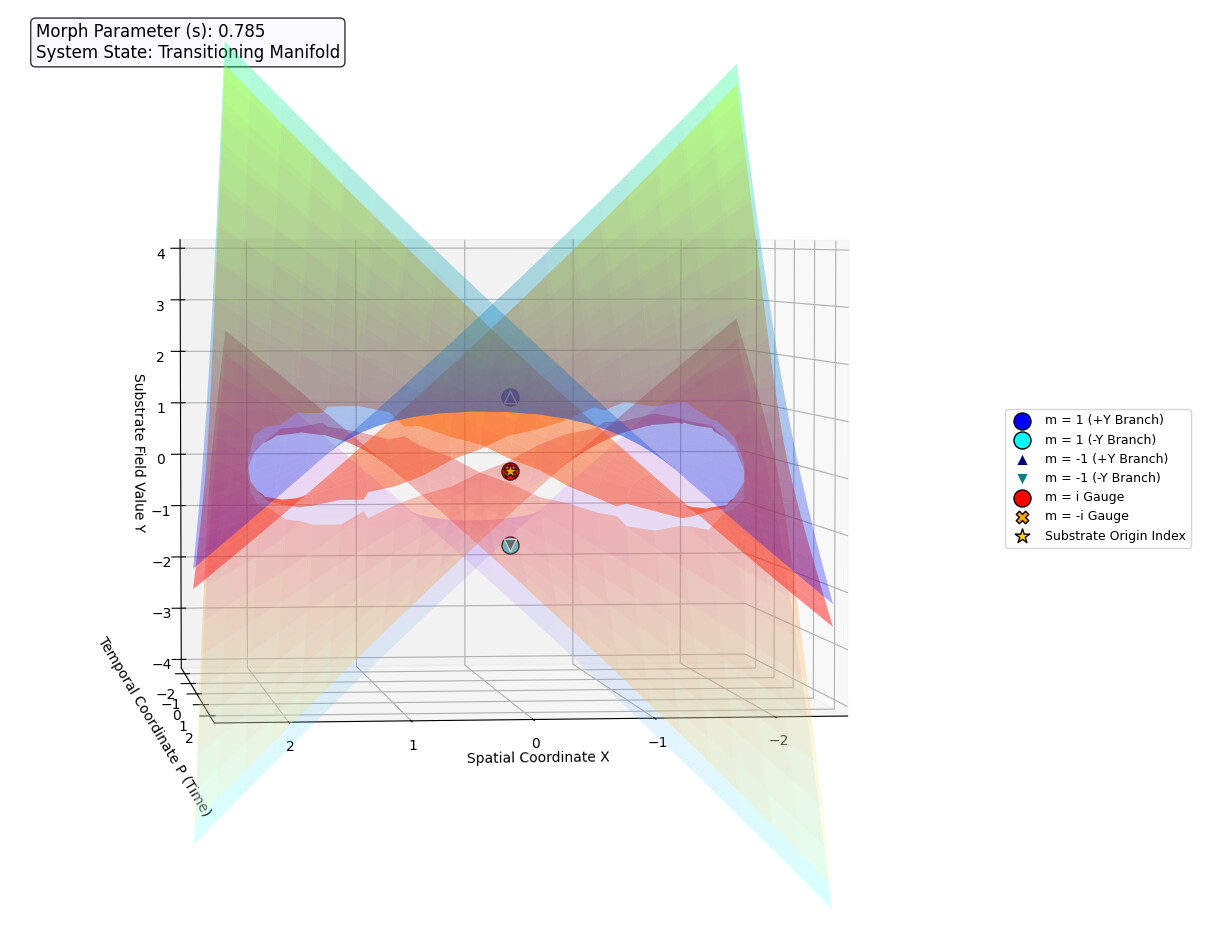
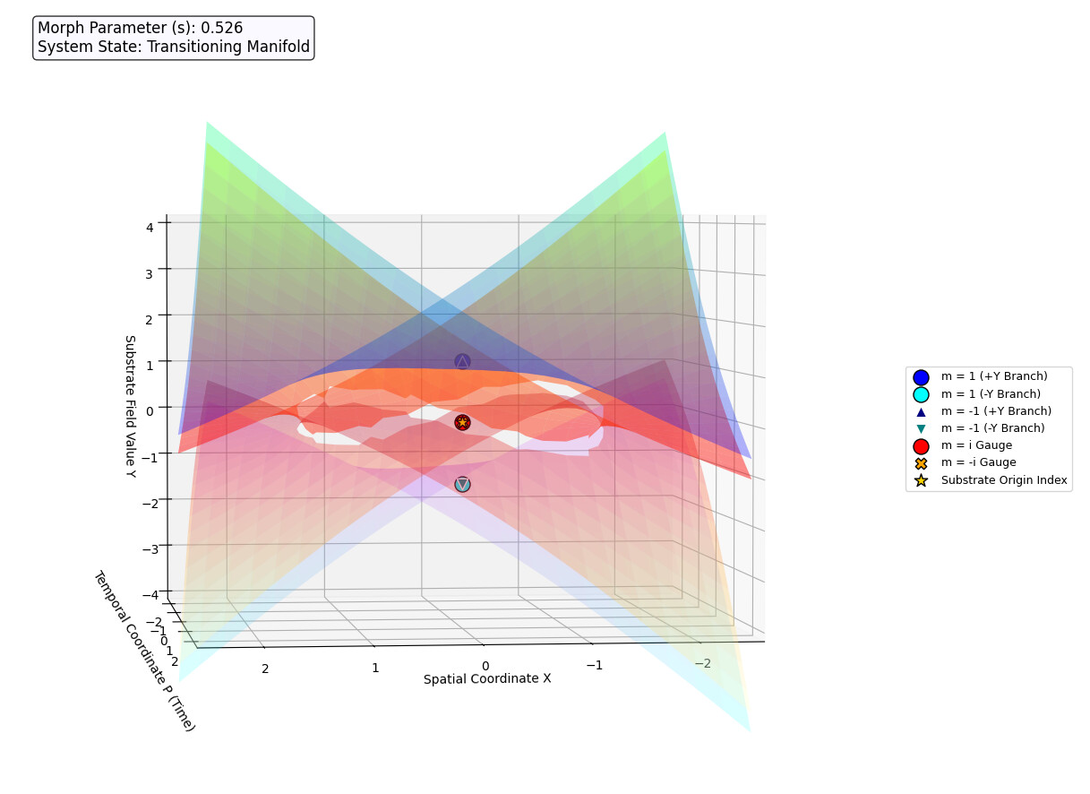
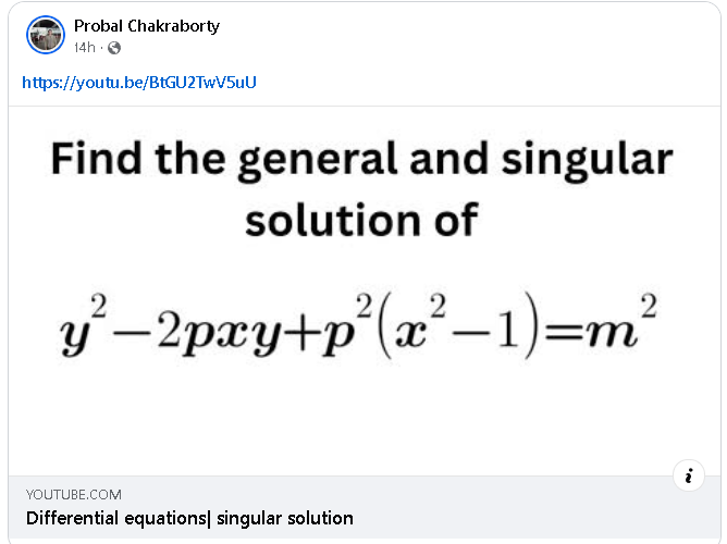





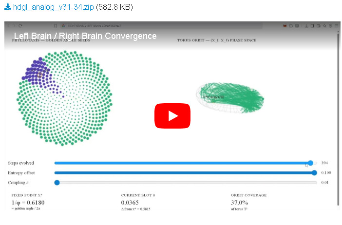
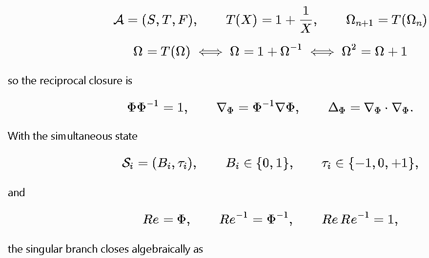

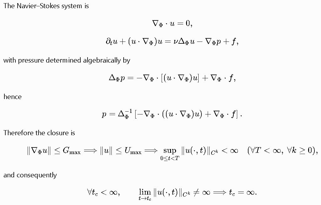
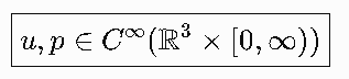

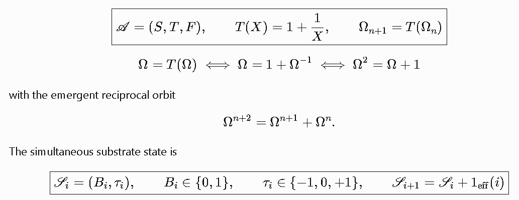
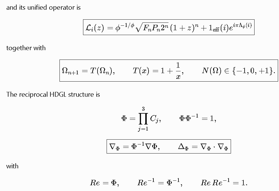
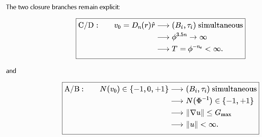
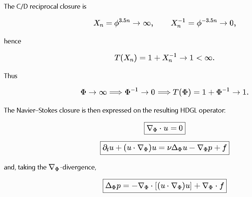
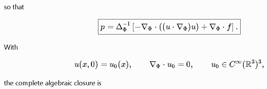

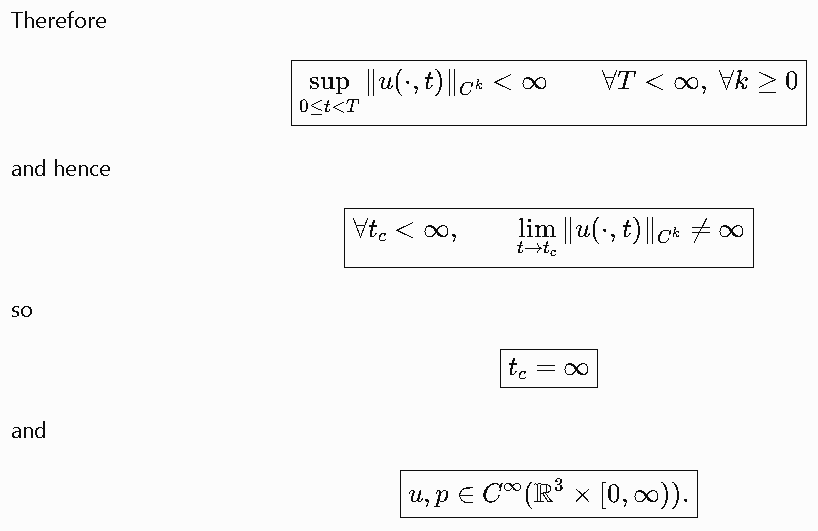
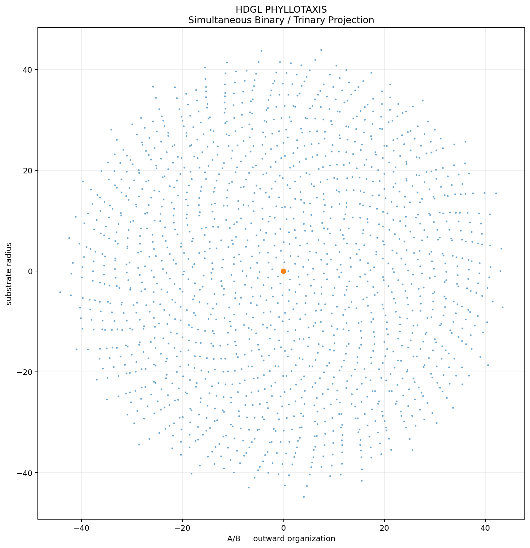
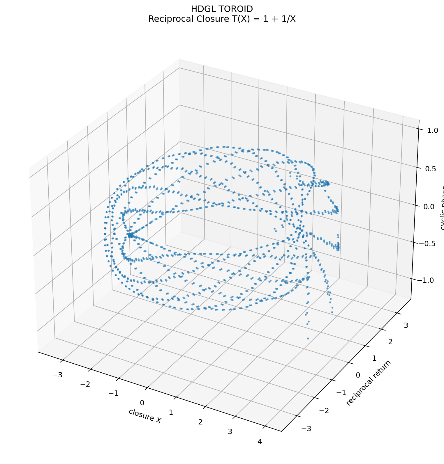
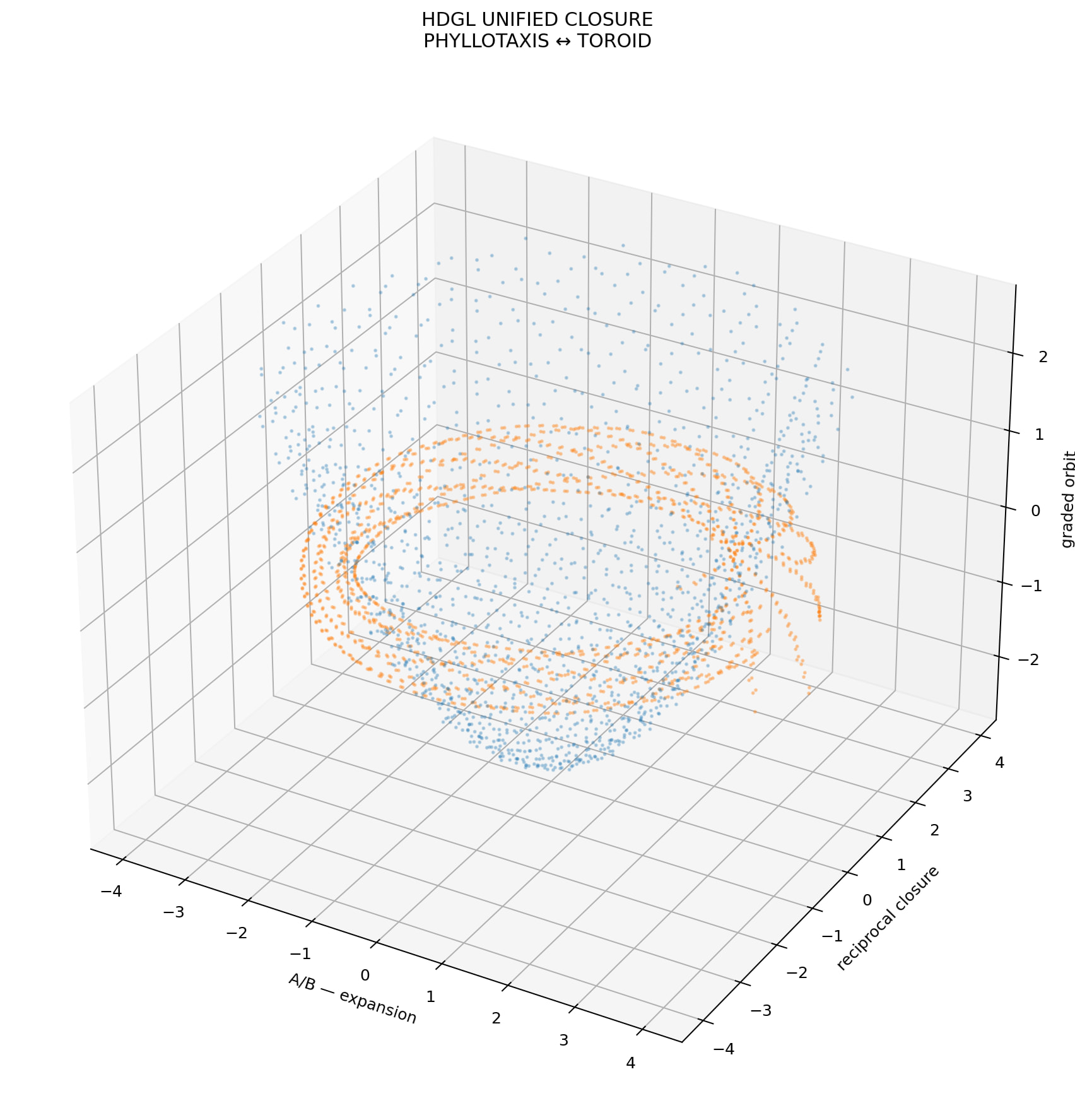
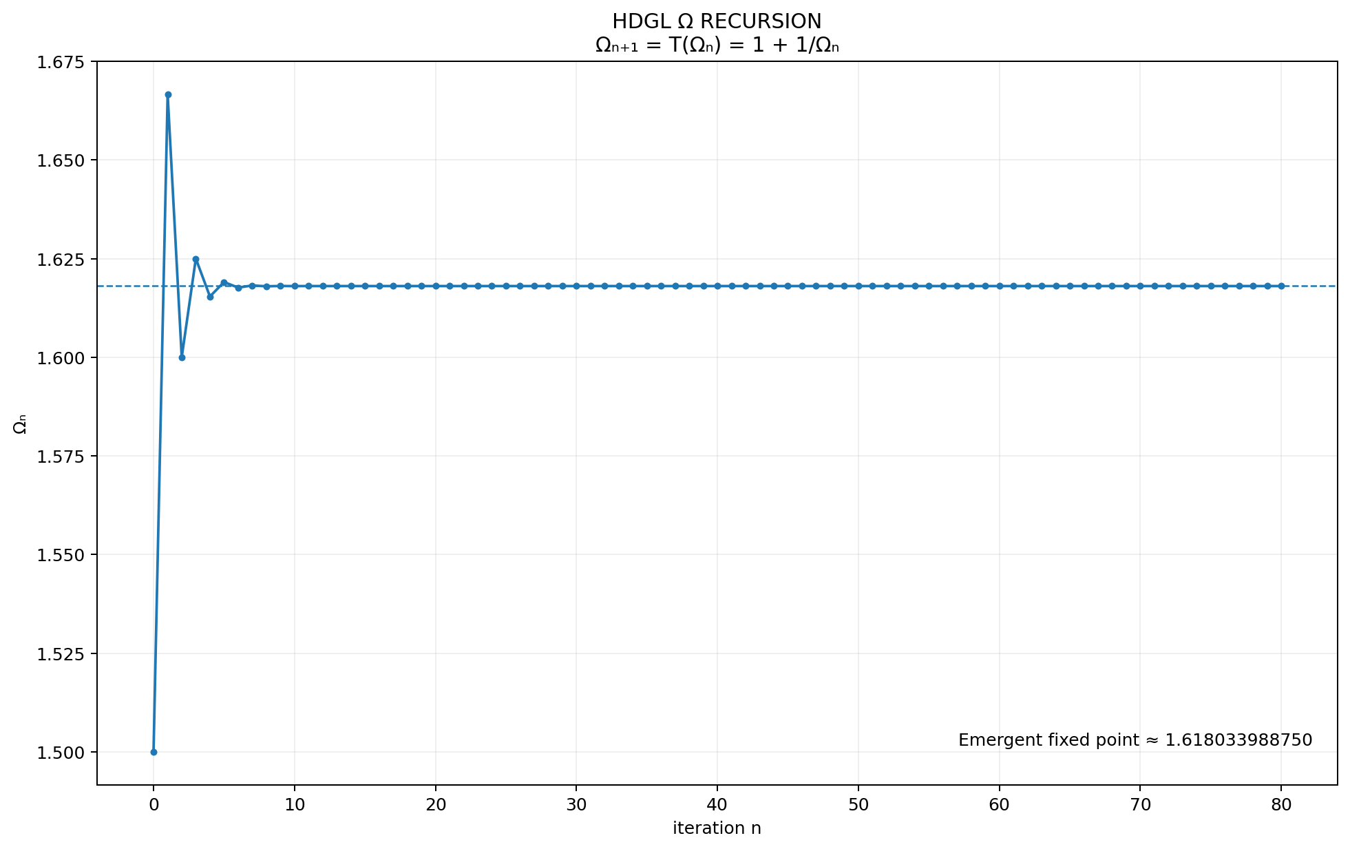
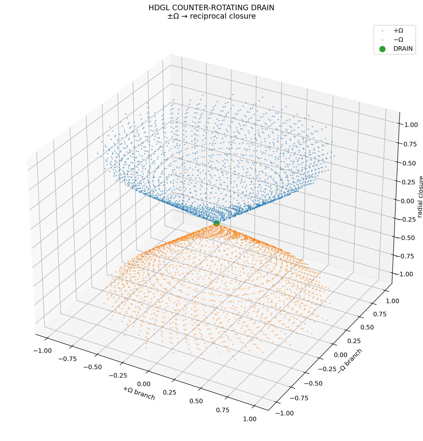
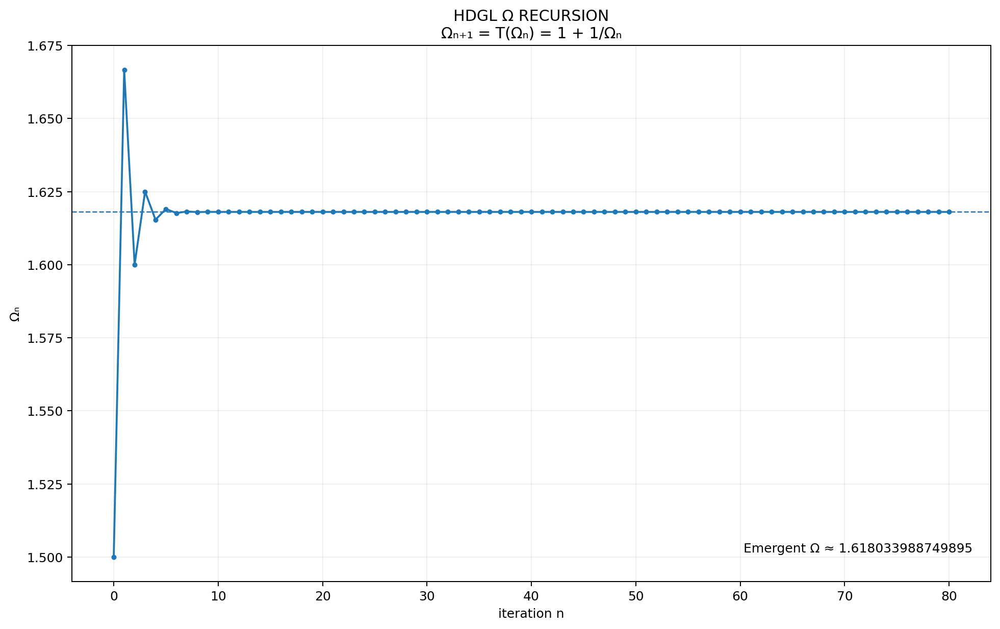
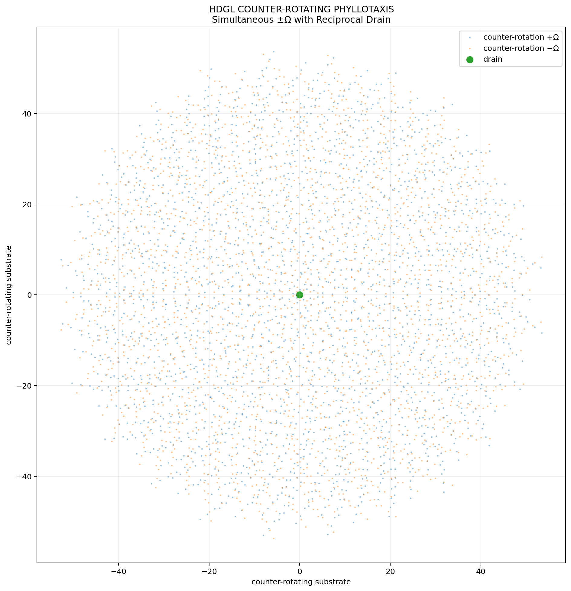
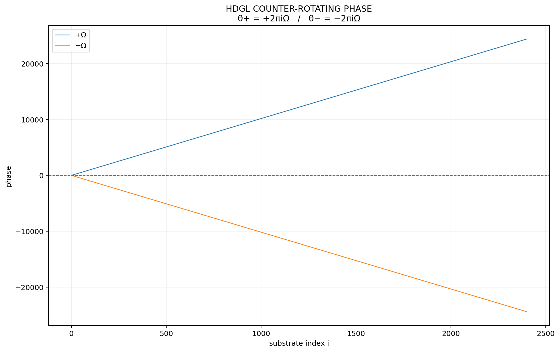
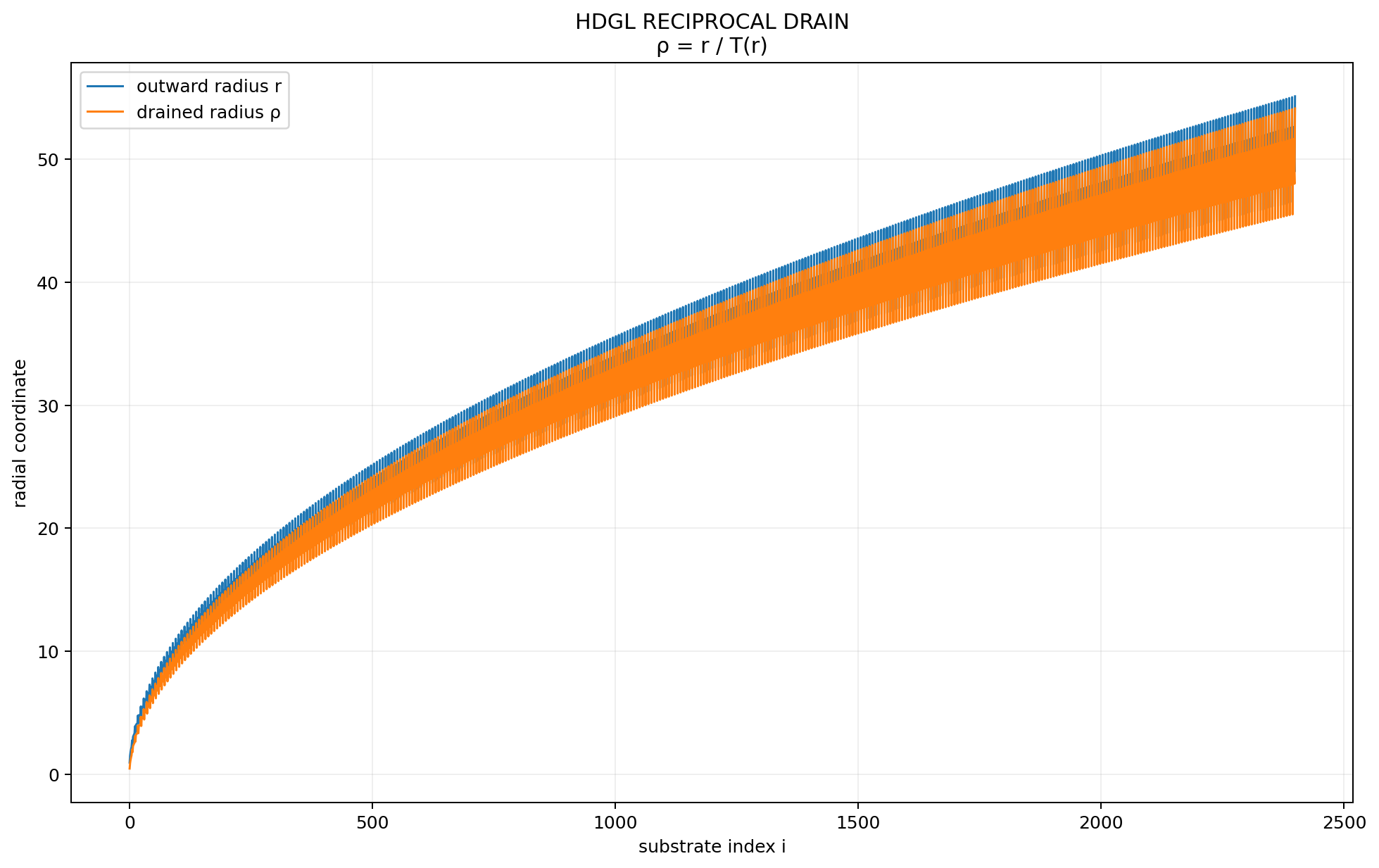
 reciprocal crossing