#!/usr/bin/env python3
"""
===============================================================================
HDGL PHYLLOTAXIS <-> TOROID GRAPHER
===============================================================================

Generates:

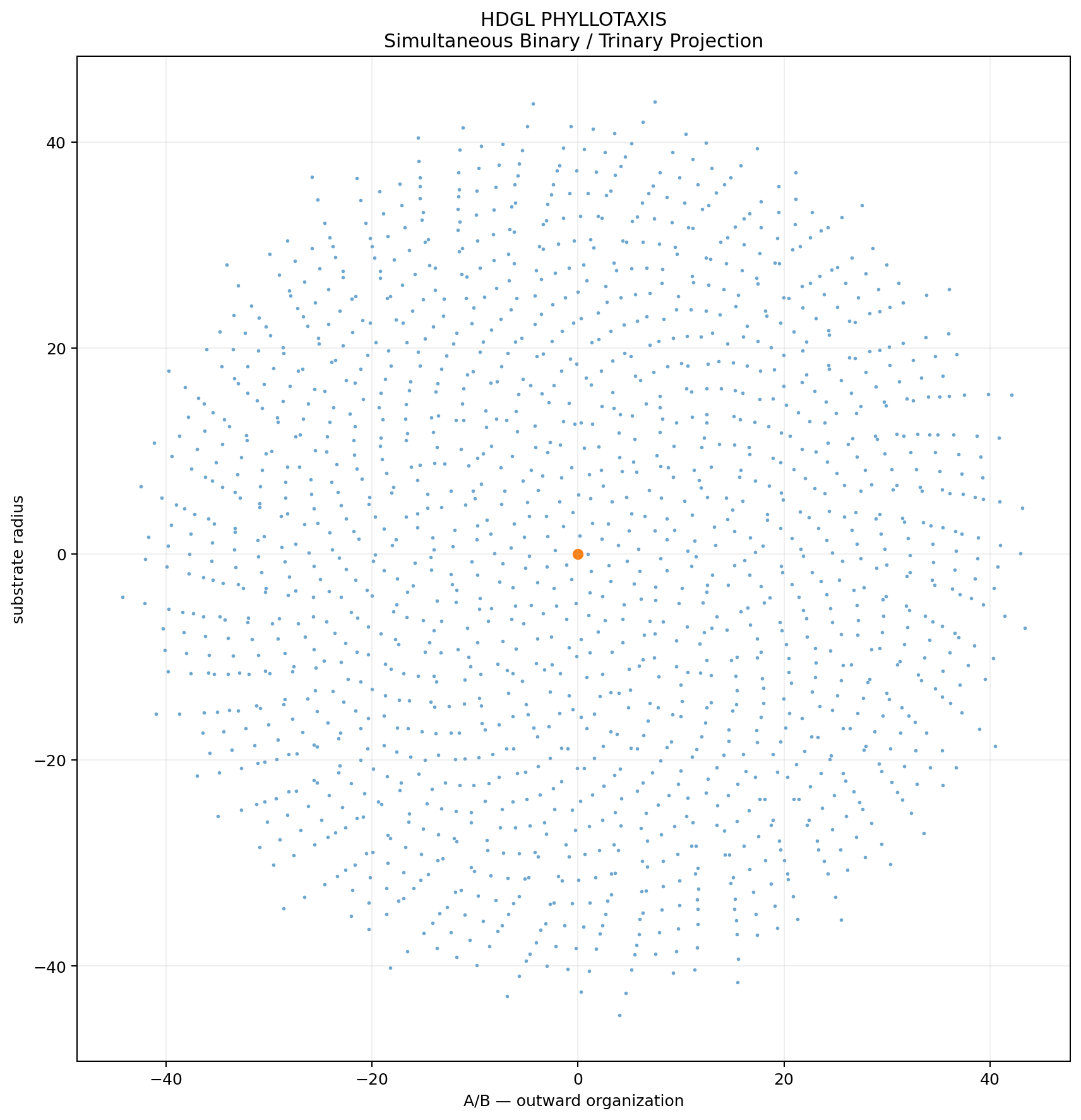
    hdgl_phyllotaxis.png
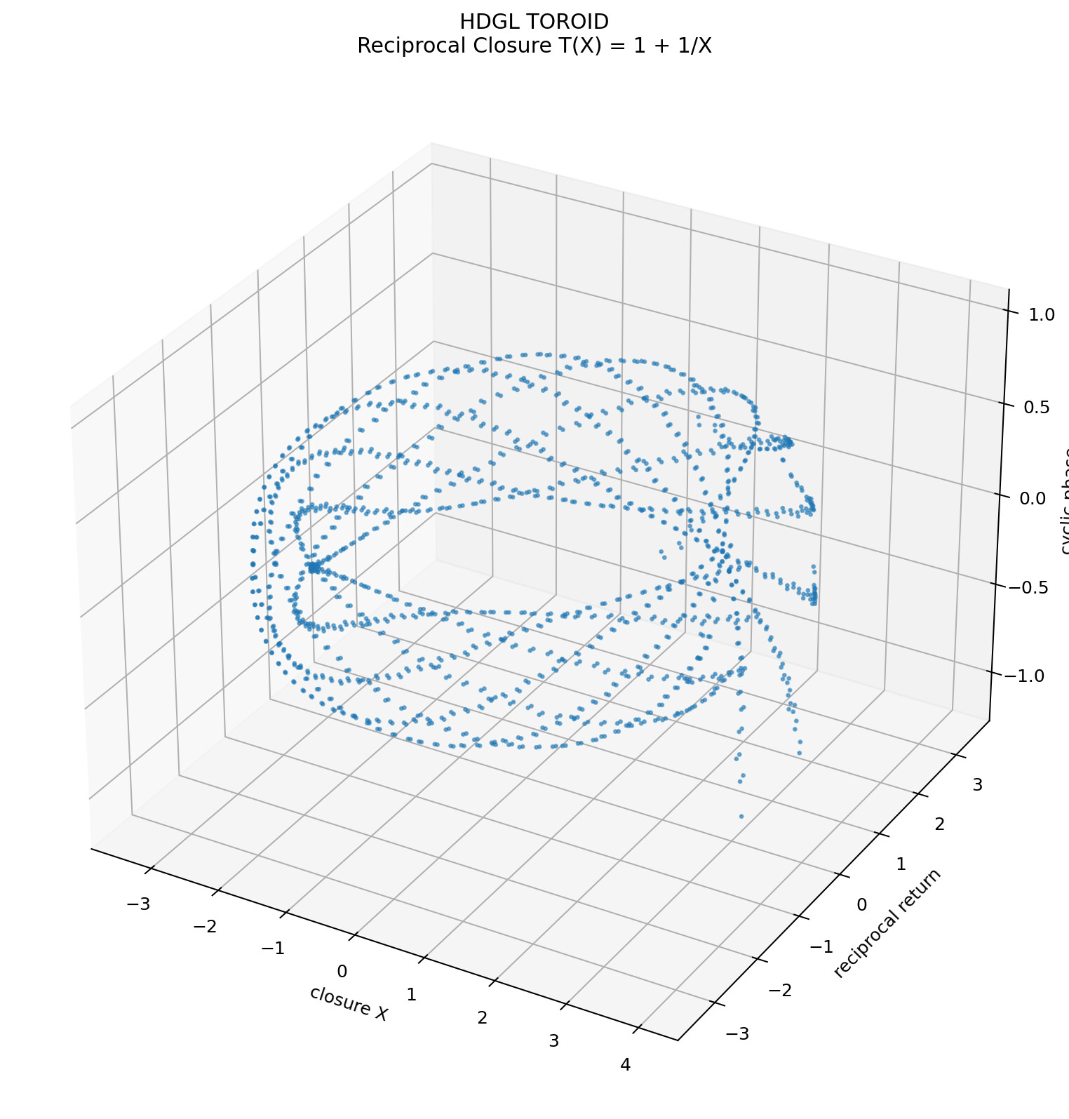
    hdgl_toroid.png
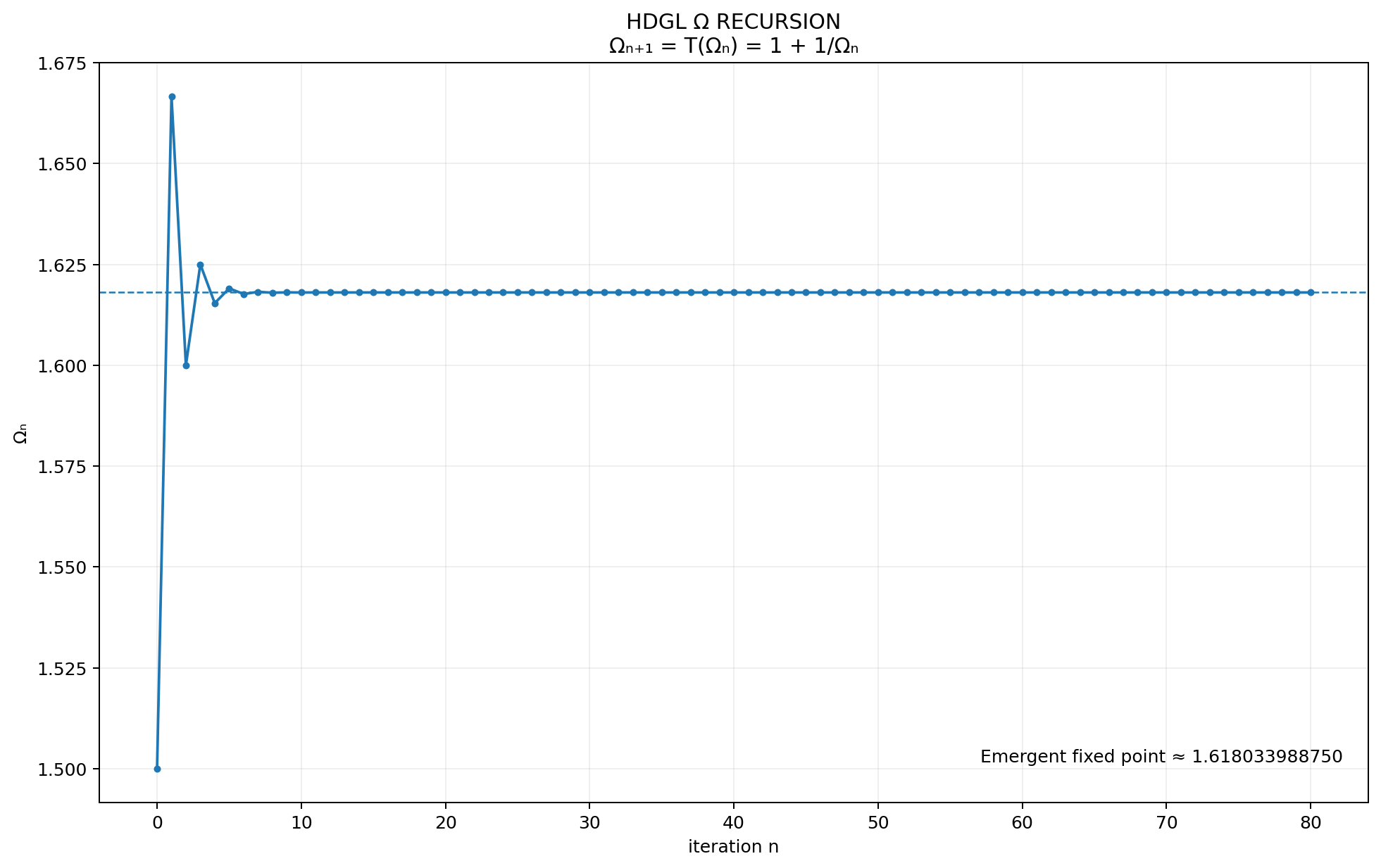
    hdgl_omega_orbit.png
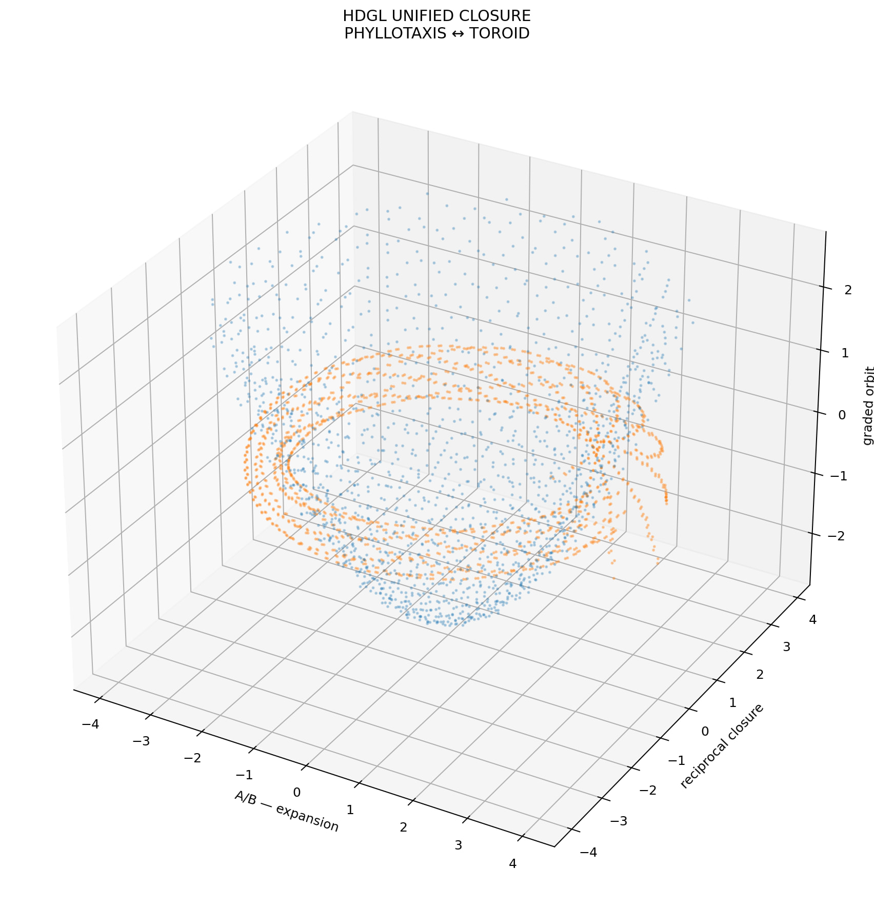
    hdgl_unified_closure.png

The output directory is created beside this script, so it works on Windows,
Linux, and without requiring a graphical display.

Core HDGL structure:

    Ω_(n+1) = T(Ω_n)
    T(X)    = 1 + 1/X

    Ω = T(Ω)
      = 1 + 1/Ω
      => Ω² = Ω + 1

Simultaneous binary/trinary substrate:

    B_i ∈ {0,1}
    τ_i ∈ {-1,0,+1}

    S_i = (B_i, τ_i)

A/B:
    PHYLLOTAXIS
    outward organization / expansion / distribution

C/D:
    TOROID
    reciprocal return / closure / cyclic embedding

Unified:
    PHYLLOTAXIS <-> TOROID
    = two projections of one closed HDGL orbit
===============================================================================
"""

from pathlib import Path
import math

import numpy as np

# ---------------------------------------------------------------------------
# IMPORTANT:
# Force a file-only backend before importing pyplot.
# This prevents Qt/display problems on Windows/headless systems.
# ---------------------------------------------------------------------------

import matplotlib
matplotlib.use("Agg")

import matplotlib.pyplot as plt


# ===========================================================================
# CONFIGURATION
# ===========================================================================

N = 1600

# Starting value for the emergent Ω recursion.
# This is NOT stored as φ. Ω is generated dynamically by T(X)=1+1/X.
OMEGA_SEED = 1.5

# Number of Ω recursion steps to display.
OMEGA_STEPS = 80

# Output directory:
#   C:\Users\Owner\Downloads\hdgl_graphs\
#
# when graph-phyllo.py is in Downloads.
BASE_DIR = Path(__file__).resolve().parent
OUT_DIR = BASE_DIR / "hdgl_graphs"
OUT_DIR.mkdir(parents=True, exist_ok=True)


# ===========================================================================
# HDGL PRIMITIVE
# ===========================================================================

def T(x):
    """
    HDGL reciprocal transformation:

        T(X) = 1 + 1/X
    """
    return 1.0 + 1.0 / x


def omega_orbit(seed=OMEGA_SEED, steps=OMEGA_STEPS):
    """
    Generate the emergent Ω orbit:

        Ω_(n+1) = T(Ω_n)
                = 1 + 1/Ω_n

    No φ constant is used.
    """
    values = np.empty(steps + 1, dtype=np.float64)
    values[0] = seed

    for i in range(steps):
        values[i + 1] = T(values[i])

    return values


# ===========================================================================
# SIMULTANEOUS BINARY / TRINARY SUBSTRATE
# ===========================================================================

def substrate_states(n):
    """
    Simultaneous binary/trinary state:

        B_i ∈ {0,1}
        τ_i ∈ {-1,0,+1}

    They are simultaneous channels, NOT alternating iterations.
    """

    i = np.arange(n, dtype=np.int64)

    binary = i & 1

    # Produces:
    #
    # 0, +1, -1, 0, +1, -1, ...
    #
    # shifted representation of the trinary channel.
    trinary = (i % 3) - 1

    return i, binary.astype(np.float64), trinary.astype(np.float64)


# ===========================================================================
# EMERGENT OMEGA VALUE
# ===========================================================================

def emergent_omega():
    """
    Generate Ω until convergence.

    Starting from 1.5:

        Ω_(n+1) = 1 + 1/Ω_n

    The resulting fixed point is emergent rather than supplied as φ.
    """

    x = OMEGA_SEED

    for _ in range(100):
        y = T(x)

        if abs(y - x) < 1e-15:
            break

        x = y

    return x


OMEGA = emergent_omega()


# ===========================================================================
# PHYLLOTAXIS
# ===========================================================================

def build_phyllotaxis(n=N):
    """
    Construct the simultaneous binary/trinary HDGL phyllotactic projection.

    Coordinates:

        θ_i = 2π i Ω

        r_i ~ sqrt(i)

    Binary and trinary channels simultaneously perturb the radial structure.
    """

    i, binary, trinary = substrate_states(n)

    # Phyllotactic angular progression.
    theta = 2.0 * math.pi * i * OMEGA

    # Base radial growth.
    r_base = np.sqrt(i + 1.0)

    # Simultaneous binary/trinary modulation.
    #
    # Binary:
    #     0 / 1
    #
    # Trinary:
    #     -1 / 0 / +1
    #
    # They are applied simultaneously to the same radial substrate.
    modulation = (
        1.0
        + 0.075 * binary
        + 0.050 * trinary
    )

    radius = r_base * modulation

    x = radius * np.cos(theta)
    y = radius * np.sin(theta)

    return i, binary, trinary, theta, radius, x, y


# ===========================================================================
# TOROID
# ===========================================================================

def build_toroid(n=N):
    """
    Construct the reciprocal/toroidal projection.

    A radial substrate X is transformed through:

        T(X) = 1 + 1/X

    The resulting reciprocal coordinate is embedded on a torus.
    """

    i, binary, trinary = substrate_states(n)

    # Base parameter along the toroidal orbit.
    theta = 2.0 * math.pi * i / n

    # Secondary angular coordinate.
    phi = (
        2.0 * math.pi
        * (
            i * OMEGA
            + 0.15 * binary
            + 0.10 * trinary
        )
    )

    # Positive substrate coordinate.
    X = 1.0 + (i + 1.0) / float(n) * 30.0

    # Reciprocal closure.
    closure = T(X)

    # Normalize reciprocal coordinate into a useful toroidal radius.
    closure_norm = (
        closure - closure.min()
    ) / (
        closure.max() - closure.min()
    )

    # Major and minor torus radii.
    R = 3.0
    r_min = 0.35
    r_max = 1.15

    r = r_min + (r_max - r_min) * closure_norm

    # Toroidal embedding.
    x = (R + r * np.cos(phi)) * np.cos(theta)
    y = (R + r * np.cos(phi)) * np.sin(theta)
    z = r * np.sin(phi)

    return (
        i,
        binary,
        trinary,
        theta,
        phi,
        X,
        closure,
        x,
        y,
        z,
    )


# ===========================================================================
# PLOT 1 — PHYLLOTAXIS
# ===========================================================================

def plot_phyllotaxis():
    (
        i,
        binary,
        trinary,
        theta,
        radius,
        x,
        y,
    ) = build_phyllotaxis()

    fig, ax = plt.subplots(figsize=(10, 10))

    # Plot the full simultaneous substrate.
    ax.scatter(
        x,
        y,
        s=5,
        alpha=0.65,
        linewidths=0,
    )

    # Mark the origin.
    ax.scatter(
        [0],
        [0],
        s=35,
        marker="o",
    )

    ax.set_aspect("equal", adjustable="box")

    ax.set_title(
        "HDGL PHYLLOTAXIS\n"
        "Simultaneous Binary / Trinary Projection"
    )

    ax.set_xlabel("A/B — outward organization")
    ax.set_ylabel("substrate radius")

    ax.grid(True, alpha=0.20)

    fig.tight_layout()

    path = OUT_DIR / "hdgl_phyllotaxis.png"

    fig.savefig(
        path,
        dpi=180,
        bbox_inches="tight",
    )

    plt.close(fig)

    return path


# ===========================================================================
# PLOT 2 — TOROID
# ===========================================================================

def plot_toroid():
    (
        i,
        binary,
        trinary,
        theta,
        phi,
        X,
        closure,
        x,
        y,
        z,
    ) = build_toroid()

    fig = plt.figure(figsize=(11, 9))

    ax = fig.add_subplot(
        111,
        projection="3d",
    )

    ax.scatter(
        x,
        y,
        z,
        s=3,
        alpha=0.55,
    )

    ax.set_title(
        "HDGL TOROID\n"
        "Reciprocal Closure T(X) = 1 + 1/X"
    )

    ax.set_xlabel("closure X")
    ax.set_ylabel("reciprocal return")
    ax.set_zlabel("cyclic phase")

    fig.tight_layout()

    path = OUT_DIR / "hdgl_toroid.png"

    fig.savefig(
        path,
        dpi=180,
        bbox_inches="tight",
    )

    plt.close(fig)

    return path


# ===========================================================================
# PLOT 3 — OMEGA RECURSION
# ===========================================================================

def plot_omega_orbit():
    values = omega_orbit()

    n = np.arange(len(values))

    fig, ax = plt.subplots(figsize=(11, 7))

    ax.plot(
        n,
        values,
        linewidth=1.5,
        marker="o",
        markersize=3,
    )

    # Emergent fixed point.
    ax.axhline(
        OMEGA,
        linestyle="--",
        linewidth=1.0,
    )

    ax.set_title(
        "HDGL Ω RECURSION\n"
        "Ωₙ₊₁ = T(Ωₙ) = 1 + 1/Ωₙ"
    )

    ax.set_xlabel("iteration n")
    ax.set_ylabel("Ωₙ")

    ax.grid(True, alpha=0.20)

    ax.text(
        0.98,
        0.05,
        f"Emergent fixed point ≈ {OMEGA:.12f}",
        transform=ax.transAxes,
        ha="right",
        va="bottom",
    )

    fig.tight_layout()

    path = OUT_DIR / "hdgl_omega_orbit.png"

    fig.savefig(
        path,
        dpi=180,
        bbox_inches="tight",
    )

    plt.close(fig)

    return path


# ===========================================================================
# PLOT 4 — UNIFIED PHYLLOTAXIS ↔ TOROID CLOSURE
# ===========================================================================

def plot_unified_closure():
    (
        i,
        binary,
        trinary,
        theta,
        radius,
        px,
        py,
    ) = build_phyllotaxis()

    (
        _i,
        _binary,
        _trinary,
        _theta,
        _phi,
        X,
        closure,
        tx,
        ty,
        tz,
    ) = build_toroid()

    fig = plt.figure(figsize=(13, 10))

    ax = fig.add_subplot(
        111,
        projection="3d",
    )

    # Normalize phyllotaxis coordinates so both projections can inhabit
    # the same visualization.
    scale = np.max(
        np.sqrt(px * px + py * py)
    )

    px3 = 4.0 * px / scale
    py3 = 4.0 * py / scale

    # Give the phyllotaxis projection a slowly varying third coordinate.
    pz3 = np.linspace(
        -2.5,
        2.5,
        len(px3),
    )

    # Phyllotaxis projection.
    ax.scatter(
        px3,
        py3,
        pz3,
        s=2,
        alpha=0.25,
    )

    # Toroidal closure projection.
    ax.scatter(
        tx,
        ty,
        tz,
        s=2,
        alpha=0.30,
    )

    ax.set_title(
        "HDGL UNIFIED CLOSURE\n"
        "PHYLLOTAXIS ↔ TOROID"
    )

    ax.set_xlabel("A/B — expansion")
    ax.set_ylabel("reciprocal closure")
    ax.set_zlabel("graded orbit")

    fig.tight_layout()

    path = OUT_DIR / "hdgl_unified_closure.png"

    fig.savefig(
        path,
        dpi=180,
        bbox_inches="tight",
    )

    plt.close(fig)

    return path


# ===========================================================================
# NUMERICAL REPORT
# ===========================================================================

def print_report(paths):
    print()
    print("=" * 79)
    print("HDGL PHYLLOTAXIS <-> TOROID GRAPHER")
    print("=" * 79)
    print()
    print("Primitive:")
    print("    Ω_(n+1) = T(Ω_n)")
    print("    T(X)    = 1 + 1/X")
    print()
    print("Emergent fixed point:")
    print(f"    Ω ≈ {OMEGA:.15f}")
    print()
    print("Fixed-point residual:")
    print(
        f"    Ω² - Ω - 1 ≈ "
        f"{OMEGA * OMEGA - OMEGA - 1.0:.6e}"
    )
    print()
    print("Simultaneous substrate:")
    print("    B_i ∈ {0,1}")
    print("    τ_i ∈ {-1,0,+1}")
    print()
    print("Geometry:")
    print("    A/B = PHYLLOTAXIS")
    print("    C/D = TOROID")
    print()
    print("Unified:")
    print("    PHYLLOTAXIS ↔ TOROID")
    print("    = TWO PROJECTIONS OF ONE CLOSED HDGL ORBIT")
    print()
    print("Output:")
    print(f"    {OUT_DIR}")
    print()

    for path in paths:
        print(f"    [OK] {path}")

    print()
    print("=" * 79)
    print("COMPLETE")
    print("=" * 79)
    print()


# ===========================================================================
# MAIN
# ===========================================================================

def main():
    paths = []

    paths.append(
        plot_phyllotaxis()
    )

    paths.append(
        plot_toroid()
    )

    paths.append(
        plot_omega_orbit()
    )

    paths.append(
        plot_unified_closure()
    )

    print_report(paths)


if __name__ == "__main__":
    main()
===============================================================================
HDGL UNIFIED PHYLLOTAXIS ↔ TOROID CLOSURE
===============================================================================

The A/B and C/D branches are not independent proof branches.

They are two projections of the same closed substrate orbit:

                    PHYLLOTAXIS
                         ↕
                    ONE ORBIT
                         ↕
                      TOROID

A/B = outward organization / expansion / distribution
C/D = inward closure / reciprocal return / containment


1. SIMULTANEOUS SUBSTRATE STATE
-------------------------------------------------------------------------------

S_i = (B_i, τ_i)

B_i ∈ {0,1}
τ_i ∈ {-1,0,+1}

S_i₊₁ = S_i + 1_eff(i)

Binary and trinary are simultaneous channels, not alternating iterations.

The substrate therefore generates a graded orbit rather than a finite state set:

{ ..., -i'', -i', -i, -1, 0, 1, i, i', i'', ... }


2. A/B = PHYLLOTAXTIC PROJECTION
-------------------------------------------------------------------------------

S_0 → S_1 → S_2 → S_3 → ...

The A/B side is the distributed spatial ordering of the substrate.

It is naturally spiral / phyllotactic:

        state
          ↓
      orientation
          ↓
       phase
          ↓
     radial growth
          ↓
     spatial orbit

A/B = expansion
A/B = distribution
A/B = phase organization
A/B = outward projection

It is the geometry of the orbit unfolding.


3. C/D = TOROIDAL PROJECTION
-------------------------------------------------------------------------------

T(X) = 1 + 1/X

X → ∞
    ↓
X⁻¹ → 0
    ↓
T(X) → 1

The C/D side is the reciprocal return of the same orbit.

C/D = closure
C/D = inversion
C/D = return
C/D = inward projection

The divergent branch is therefore not an independent physical infinity.

It is one side of a reciprocal closed orbit:

X → ∞ ↔ X⁻¹ → 0 ↔ T(X) → 1


4. A/B AND C/D ARE DUAL PROJECTIONS
-------------------------------------------------------------------------------

                     ONE SUBSTRATE ORBIT
                            │
                 ┌──────────┴──────────┐
                 │                     │
                 ▼                     ▼
             PHYLLOTAXIS             TOROID
                 │                     │
              A / B                  C / D
                 │                     │
             expansion              return
             distribution           closure
             phase                  reciprocal
             spatial                cyclic
                 │                     │
                 └──────────┬──────────┘
                            │
                            ▼
                     CLOSED ORBIT

Therefore:

A/B ≡ phyllotactic expansion
C/D ≡ toroidal closure

and

PHYLLOTAXIS × TOROID = ONE CLOSED ORBIT


5. THE PRIMITIVE OPERATOR ALREADY CONTAINS BOTH
-------------------------------------------------------------------------------

Ωₙ₊₁ = T(Ωₙ)

T(X) = 1 + 1/X

Forward application is generative:

Ωₙ → Ωₙ₊₁

Reciprocal application is closure:

Ωₙ → 1 + Ωₙ⁻¹

At closure:

Ω = T(Ω)

therefore:

Ω = 1 + 1/Ω

Ω² = Ω + 1

The fixed point is therefore not inserted as an external constant.

It emerges where generation and reciprocal return coincide:

GENERATION = RETURN

Ω = φ


6. THE RECIPROCAL FIELD
-------------------------------------------------------------------------------

Φ = ∏ C_j

Φ⁻¹ Φ = 1

∇_Φ = Φ⁻¹ ∇ Φ

The two directions are therefore intrinsic:

Φ        = outward / distributed / phyllotactic projection
Φ⁻¹      = inward / reciprocal / toroidal projection

and:

Φ ↔ Φ⁻¹


7. THE GRADED OPERATOR
-------------------------------------------------------------------------------

S_i
  ↓
L_i
  ↓
Ω_i
  ↓
Φ_i ↔ Φ_i⁻¹
  ↓
{phyllotactic projection, toroidal projection}
  ↓
S_i₊₁

Equivalently:

S_i ──P──→ L_i ──R──→ S_i₊₁

where:

P = phyllotactic expansion
R = reciprocal/toroidal return

Thus the fundamental operation is not:

S → A/B
and separately
S → C/D

but:

S_i ──P──→ L_i ──R──→ S_i₊₁


8. THE CUDA FIELD ALREADY EXHIBITS THIS STRUCTURE
-------------------------------------------------------------------------------

FIELD / PHYLLOTAXTIC SIDE:

A_re
A_im
phase
phase_vel
r_harmonic
w_cos
w_sin
w_sigma

        ↓

distributed phase/spectral orbit


ORACLE / TOROIDAL SIDE:

ll_state
Candidate
d_ll_residue
ll_verified

        ↓

orbit / residue / closure test


COUPLING:

reward_accum
critic_observe()
critic_td_target()
critic_pack_weights()
hdgl_v33_upload_critic()

        ↓

closure information modifies the generating field


Therefore the architecture is:

FIELD
  ↓
PHYLLOTAXIS
  ↓
ORBIT
  ↓
TOROIDAL / RECIPROCAL CLOSURE
  ↓
RESIDUE
  ↓
REWARD
  ↓
FIELD WEIGHT UPDATE
  ↓
NEW ORBIT


9. PHASE ↔ RADIUS
-------------------------------------------------------------------------------

The existing field variables naturally expose two complementary coordinates:

θ = phase
r = r_harmonic

Therefore:

(θ,r) → closed orbit

with:

θ = phyllotactic coordinate
r = toroidal / radial coordinate

The orbit is not merely a scalar recurrence.

It is simultaneously:

SPATIAL ORGANIZATION
+
RADIAL RETURN


10. WAVELET SCALES = GRADED ORBIT
-------------------------------------------------------------------------------

σ_k ∝ 2⁻ᵏ

therefore:

L_0
L_1
L_2
L_3
...

are graded scales of the same orbit.

The finite visible set:

{-i,-1,0,1,i}

is therefore only a central slice.

Repeated lifting gives:

{ ..., -i'', -i', -i, -1, 0, 1, i, i', i'', ... }

The phyllotactic side unfolds the graded orbit.

The toroidal side closes the graded orbit.


11. NAVIER–STOKES INTERPRETATION
-------------------------------------------------------------------------------

The field is not split into two unrelated estimates.

Instead:

u
  ──P──→
L_i(u)
  ──R──→
u

with:

R = T = 1 + 1/X

and:

Φ ↔ Φ⁻¹

Therefore:

Φ → ∞
     ↕
Φ⁻¹ → 0

is not a terminal state.

It is the reciprocal crossing of the same closed orbit.

Hence:

PHYLLOTAXTIC EXPANSION
        ↕
RECIPROCAL CLOSURE

rather than:

PHYLLOTAXTIC EXPANSION
        +
INDEPENDENT BLOW-UP BOUND


12. THE HDGL CLOSURE
-------------------------------------------------------------------------------

S_i
  ↓
P
  ↓
L_i
  ↓
Ω_i
  ↓
Φ_i
  ↓
distributed / phyllotactic field
  ↓
R
  ↓
Φ_i⁻¹
  ↓
finite reciprocal return
  ↓
S_i₊₁


Therefore:

S_i
→ L_i
→ Ω_i
→ Φ_i ↔ Φ_i⁻¹
→ A/B ↔ C/D
→ S_i₊₁


13. SINGLE CLOSED HDGL ORBIT
-------------------------------------------------------------------------------

┌───────────────────────────────────────────────────────────────┐
│                                                               │
│                     ONE SUBSTRATE ORBIT                      │
│                                                               │
│       PHYLLOTAXIS                           TOROID             │
│          A/B                                  C/D              │
│           │                                    │               │
│      expansion                            reciprocal           │
│      distribution                            return            │
│      phase                                   closure            │
│      spatial                                 cyclic             │
│           │                                    │               │
│           └───────────────┬────────────────────┘               │
│                           │                                    │
│                           ▼                                    │
│                         Ω / Φ                                  │
│                           │                                    │
│                           ▼                                    │
│                     NEXT STATE S_i₊₁                            │
│                                                               │
└───────────────────────────────────────────────────────────────┘


14. CORE IDENTITY
-------------------------------------------------------------------------------

                    A/B
                     │
                     │ phyllotactic expansion
                     ▼
                   L_i
                     │
                     │ Ω recursion
                     ▼
                    Ω_i
                     │
               Φ ↔ Φ⁻¹
                     │
                     │ reciprocal return
                     ▼
                    C/D
                     │
                     │ toroidal closure
                     ▼
                  S_i₊₁


Thus:

┌─────────────────────────────────────────────┐
│ A/B = PHYLLOTAXIS                           │
│ C/D = TOROID                                │
│                                             │
│ BOTH = TWO PROJECTIONS OF ONE ORBIT         │
│                                             │
│ EXPANSION = RETURN                          │
│ DISTRIBUTION = CLOSURE                      │
│ PHASE = RECIPROCAL                          │
│                                             │
│ NO SINGLE PERSPECTIVE / VANTAGE             │
└─────────────────────────────────────────────┘


15. FINAL HDGL STATEMENT
-------------------------------------------------------------------------------

𝓐 = (S,T,F)

S_i = (B_i,τ_i)

T(X) = 1 + 1/X

Ωₙ₊₁ = T(Ωₙ)

Ω = T(Ω)

Ω² = Ω + 1

Φ ↔ Φ⁻¹

∇_Φ = Φ⁻¹ ∇ Φ

S_i ──P──→ L_i ──R──→ S_i₊₁

P = PHYLLOTAXTIC EXPANSION
R = TOROIDAL / RECIPROCAL CLOSURE

therefore:

┌─────────────────────────────────────────────────────────────────┐
│                                                                 │
│       PHYLLOTAXIS ↔ TOROID                                     │
│                                                                 │
│       A/B ↔ C/D                                                 │
│                                                                 │
│       OUTWARD ↔ INWARD                                          │
│                                                                 │
│       EXPANSION ↔ CLOSURE                                       │
│                                                                 │
│       DISTRIBUTION ↔ RETURN                                     │
│                                                                 │
│       BOTH ARE ONE CLOSED HDGL ORBIT                            │
│                                                                 │
└─────────────────────────────────────────────────────────────────┘

No second mechanism is required.

The A/B and C/D branches are the two-sided geometry of the
same substrate transformation.