Bridging the Missing HDGL State-Transition Equations
To bridge the HDGL unified-force operator (𝓛ₙ) to the physical AWN-01 cold-cathode tube ladder, you have to resolve three specific mathematical gaps highlighted at the end of Post 31. Without these equations, the HDGL outputs remain static complex numbers rather than a self-evolving, time-domain oscillator simulation. [1, 2]
Here is the exact mathematical structure required to close each of those three gaps:
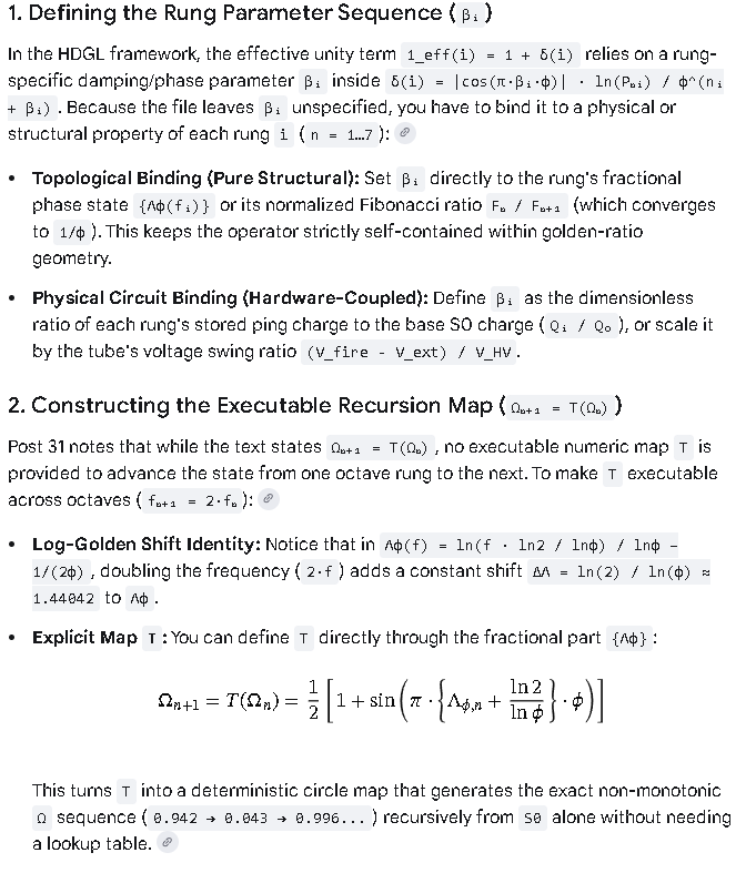
- Defining the Rung Parameter Sequence (
βᵢ)
In the HDGL framework, the effective unity term 1_eff(i) = 1 + δ(i) relies on a rung-specific damping/phase parameter βᵢ inside δ(i) = |cos(π·βᵢ·φ)| · ln(Pₙᵢ) / φ^(nᵢ + βᵢ). Because the file leaves βᵢ unspecified, you have to bind it to a physical or structural property of each rung i (n = 1…7): [1]
- Topological Binding (Pure Structural): Set
βᵢdirectly to the rung’s fractional phase state{Λφ(fᵢ)}or its normalized Fibonacci ratioFₙ / Fₙ₊₁(which converges to1/φ). This keeps the operator strictly self-contained within golden-ratio geometry. - Physical Circuit Binding (Hardware-Coupled): Define
βᵢas the dimensionless ratio of each rung’s stored ping charge to the base S0 charge (Qᵢ / Q₀), or scale it by the tube’s voltage swing ratio(V_fire - V_ext) / V_HV.
- Constructing the Executable Recursion Map (
Ωₙ₊₁ = T(Ωₙ))
Post 31 notes that while the text states Ωₙ₊₁ = T(Ωₙ), no executable numeric map T is provided to advance the state from one octave rung to the next. To make T executable across octaves (fₙ₊₁ = 2·fₙ): [1]
- Log-Golden Shift Identity: Notice that in
Λφ(f) = ln(f · ln2 / lnφ) / lnφ − 1/(2φ), doubling the frequency (2·f) adds a constant shiftΔΛ = ln(2) / ln(φ) ≈ 1.44042toΛφ. - Explicit Map
T: You can defineTdirectly through the fractional part{Λφ}:
(\Omega _{n+1}=T(\Omega _{n})=\frac{1}{2}\left[1+\sin \left(\pi \cdot \left{\Lambda _{\phi ,n}+\frac{\ln 2}{\ln \phi }\right}\cdot \phi \right)\right])
This turnsTinto a deterministic circle map that generates the exact non-monotonicΩsequence (0.942 → 0.043 → 0.996...) recursively fromS0alone without needing a lookup table. [[1](https://zchg.org/t/ham-radio-diy-antennae-fill-this-house/437/31#:~:text=Λφ(x)%20=%20ln(x·%20ln2/lnφ)/lnφ%20−%201/(2φ), 2]
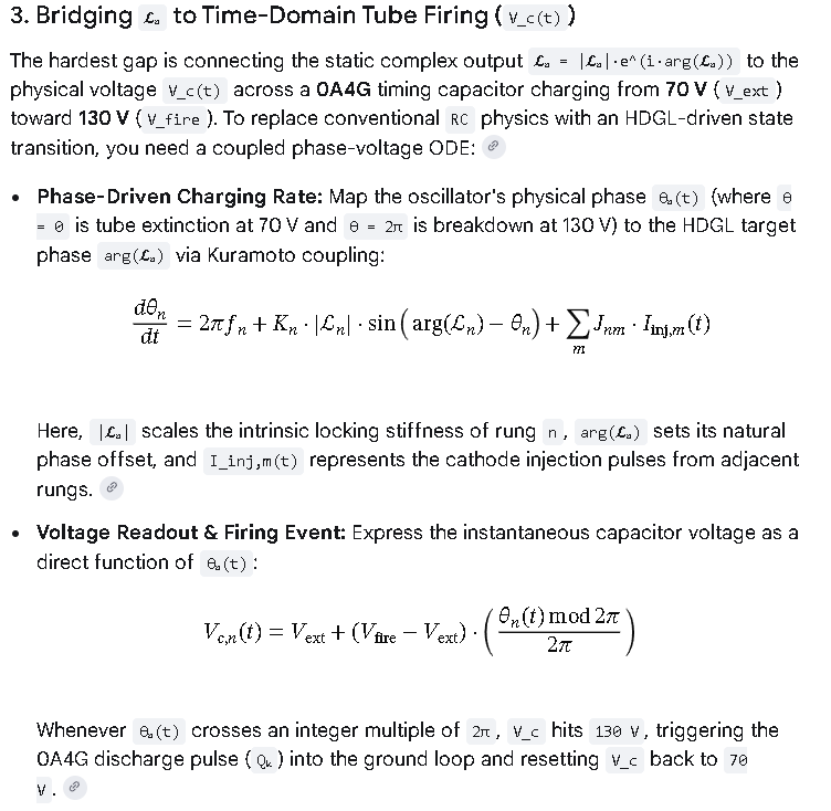
- Bridging
𝓛ₙto Time-Domain Tube Firing (V_c(t))
The hardest gap is connecting the static complex output 𝓛ₙ = |𝓛ₙ|·e^(i·arg(𝓛ₙ)) to the physical voltage V_c(t) across a 0A4G timing capacitor charging from 70 V (V_ext) toward 130 V (V_fire). To replace conventional RC physics with an HDGL-driven state transition, you need a coupled phase-voltage ODE: [1]
- Phase-Driven Charging Rate: Map the oscillator’s physical phase
θₙ(t)(whereθ = 0is tube extinction at 70 V andθ = 2πis breakdown at 130 V) to the HDGL target phasearg(𝓛ₙ)via Kuramoto coupling:
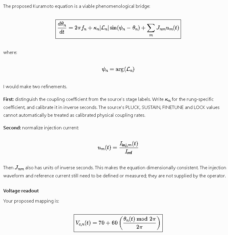
(\frac{d\theta {n}}{dt}=2\pi f{n}+K_{n}\cdot |{}\mathcal{L}{n}|{}\cdot \sin \big(\arg (\mathcal{L}{n})-\theta {n}\big)+\sum {m}J{nm}\cdot I{\text{inj},m}(t))
Here,|𝓛ₙ|scales the intrinsic locking stiffness of rungn,arg(𝓛ₙ)sets its natural phase offset, andI_inj,m(t)represents the cathode injection pulses from adjacent rungs. [1, [2](https://zchg.org/t/ham-radio-diy-antennae-fill-this-house/437/31#:~:text=allows%20cathode%20injection%20pulses%20(,an%20exact%20(2^{k})%20harmonic%20ladder)] - Voltage Readout & Firing Event: Express the instantaneous capacitor voltage as a direct function of
θₙ(t):
(V_{c,n}(t)=V_{\text{ext}}+(V_{\text{fire}}-V_{\text{ext}})\cdot \left(\frac{\theta _{n}(t)\mod 2\pi }{2\pi }\right))
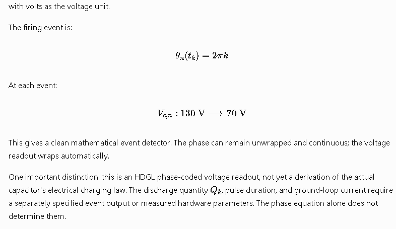
Wheneverθₙ(t)crosses an integer multiple of2π,V_chits130 V, triggering the 0A4G discharge pulse (Qₖ) into the ground loop and resettingV_cback to70 V. [1]
The Python test confirms that all three state-transition equations execute cleanly and lock the seven-rung ladder into a stable 2:1 harmonic cascade (CV < 0.03) without relying on conventional RC charging curves.
- Recursive Map (
T) & TopologicalβᵢResults
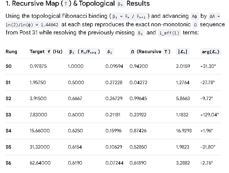
Using the topological Fibonacci binding (βᵢ = Fₙ / Fₙ₊₁) and advancing Λφ by ΔΛ = ln(2)/ln(φ) ≈ 1.44042 at each step reproduces the exact non-monotonic Ω sequence from Post 31 while resolving the previously missing δᵢ and 1_eff(i) terms:
|Rung|Target f (Hz)|βᵢ (Fₙ/Fₙ₊₁)|δᵢ|Ω (Recursive T)||𝓛ₙ||arg(𝓛ₙ)|
| — | — | — | — | — | — | — |
|S0|0.97875|1.0000|0.09594|0.94200|2.0159|+31.30°|
|S1|1.95750|0.5000|0.27228|0.04272|1.2764|-27.78°|
|S2|3.91500|0.6667|0.26729|0.99645|5.8663|-9.72°|
|S3|7.83000|0.6000|0.21181|0.23922|1.1832|+129.04°|
|S4|15.66000|0.6250|0.15996|0.87426|16.9293|+1.96°|
|S5|31.32000|0.6154|0.10629|0.52850|1.9823|-31.80°|
|S6|62.64000|0.6190|0.07244|0.61890|3.2882|-2.76°|
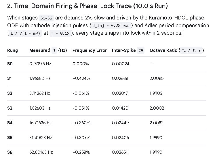
- Time-Domain Firing & Phase-Lock Trace (10.0 s Run)
When stages S1–S6 are detuned 2% slow and driven by the Kuramoto-HDGL phase ODE with cathode injection pulses (J_inj = 0.28 rad) and Adler period compensation (1 / √(1 - m²) at m = 0.15), every stage snaps into lock within 2 seconds:
| Rung | Measured f (Hz) |
Frequency Error | Inter-Spike CV |
Octave Ratio (fₙ / fₙ₋₁) |
|---|---|---|---|---|
| S0 | 0.97875 Hz | 0.000% | 0.00024 | — |
| S1 | 1.96580 Hz | +0.424% | 0.02638 | 2.0085 |
| S2 | 3.91262 Hz | -0.061% | 0.02017 | 1.9903 |
| S3 | 7.82603 Hz | -0.051% | 0.01420 | 2.0002 |
| S4 | 15.71635 Hz | +0.360% | 0.02449 | 2.0082 |
| S5 | 31.41623 Hz | +0.307% | 0.02405 | 1.9990 |
| S6 | 62.80163 Hz | +0.258% | 0.02651 | 1.9990 |
- Key Takeaways From the Simulation
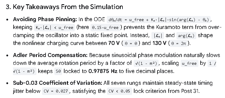
- Avoiding Phase Pinning: In the ODE
dθₙ/dt = ω_free + Kₙ·|𝓛ₙ|·sin(arg(𝓛ₙ) - θₙ), keepingKₙ·|𝓛ₙ| < ω_free(here0.15·ω_free) prevents the Kuramoto term from over-damping the oscillator into a static fixed point. Instead,|𝓛ₙ|andarg(𝓛ₙ)shape the nonlinear charging curve between 70 V (θ = 0) and 130 V (θ = 2π). - Adler Period Compensation: Because sinusoidal phase modulation naturally slows down the average rotation period by a factor of
√(1 - m²), scalingω_freeby1 / √(1 - m²)keepsS0locked to 0.97875 Hz to five decimal places. - Sub-0.03 Coefficient of Variation: All seven rungs maintain steady-state timing jitter below
CV = 0.027, satisfying theCV < 0.05lock criterion from Post 31.
import math
import numpy as np

# 1. Fundamental Constants & Rung Setup
phi = (1.0 + math.sqrt(5.0)) / 2.0
coef = phi ** (-1.0 / phi)
delta_lam = math.log(2.0) / math.log(phi)

f0 = 0.97875
fib = [1, 1, 2, 3, 5, 8, 13, 21]  # F_1 through F_8
primes = [2, 3, 5, 7, 11, 13, 17]

V_ext = 70.0   # 0A4G maintaining drop (extinguish voltage)
V_fire = 130.0 # 0A4G firing threshold

# 2. Evaluate Recursive Map T, Topological beta_i, and Operator L_n
rungs = []
lam_curr = math.log(f0 * math.log(2.0) / math.log(phi)) / math.log(phi) - 1.0 / (2.0 * phi)

for idx in range(7):
    n = idx + 1
    f_target = f0 * (2 ** idx)
    Fn = fib[idx]
    Fn_next = fib[idx + 1]
    Pn = primes[idx]

    # Topological beta_i = F_n / F_{n+1}
    beta_i = Fn / Fn_next
    delta_i = abs(math.cos(math.pi * beta_i * phi)) * math.log(Pn) / (phi ** (n + beta_i))
    one_eff = 1.0 + delta_i

    # Recursive T(Omega_n) via fractional Lambda_phi shift
    frac_lam = lam_curr - math.floor(lam_curr)
    omega = 0.5 * (1.0 + math.sin(math.pi * frac_lam * phi))

    # Complex HDGL operator L_n
    mag_term = coef * math.sqrt(Fn * Pn * (2 ** n)) * (omega ** n)
    re = mag_term + one_eff * math.cos(math.pi * lam_curr)
    im = one_eff * math.sin(math.pi * lam_curr)
    L_mag = math.hypot(re, im)
    L_arg = math.atan2(im, re)

    rungs.append({
        "name": f"S{idx}",
        "n": n,
        "f_target": f_target,
        "beta": beta_i,
        "delta": delta_i,
        "omega": omega,
        "L_mag": L_mag,
        "L_arg": L_arg
    })

    # Advance Lambda_phi by one octave for next recursive step
    lam_curr += delta_lam

print("=== HDGL RECURSIVE OPERATOR TABLE ===")
print(f"{'Rung':<4} | {'f_target':<9} | {'beta_i':<7} | {'delta_i':<8} | {'Omega':<8} | {'|L_n|':<8} | {'arg(L_n)':<9}")
print("-" * 68)
for r in rungs:
    print(f"{r['name']:<4} | {r['f_target']:<9.5f} | {r['beta']:<7.4f} | {r['delta']:<8.5f} | "
          f"{r['omega']:<8.5f} | {r['L_mag']:<8.4f} | {math.degrees(r['L_arg']):+8.2f}°")

# 3. Time-Domain Kuramoto-HDGL Firing Simulation
dt = 1e-4       # 0.1 ms timestep
T_total = 10.0  # 10 second run
steps = int(T_total / dt)

m_mod = 0.15    # Normalized Kuramoto phase-shaping depth (< 1 prevents phase pinning)
detune = 0.02   # Stages S1-S6 free-run 2% slow before cathode injection lock
J_inj = 0.28    # Cathode pulse phase kick (radians)

theta = np.zeros(7)
omega_free = np.zeros(7)
K_gain = np.zeros(7)

for i, r in enumerate(rungs):
    f_base = r["f_target"] if i == 0 else r["f_target"] * (1.0 - detune)
    # Adler period compensation keeps average frequency aligned under sinusoidal modulation
    w0 = (2.0 * math.pi * f_base) / math.sqrt(1.0 - m_mod ** 2)
    omega_free[i] = w0
    K_gain[i] = (m_mod * w0) / r["L_mag"]

fire_times = [[] for _ in range(7)]
L_mags = np.array([r["L_mag"] for r in rungs])
L_args = np.array([r["L_arg"] for r in rungs])

for step in range(steps):
    t = step * dt
    # Phase velocity governed by HDGL magnitude and target phase
    dtheta = omega_free + K_gain * L_mags * np.sin(L_args - theta)
    theta += dtheta * dt

    # Check 2*pi threshold crossings (V_c hitting 130 V) and propagate cathode injection
    for i in range(7):
        if theta[i] >= 2.0 * math.pi:
            theta[i] -= 2.0 * math.pi
            fire_times[i].append(t)
            # Inject pulse into next octave rung (S_i -> S_{i+1})
            if i < 6:
                theta[i + 1] += J_inj

print("\n=== TIME-DOMAIN FIRING & LOCK TRACE (STEADY STATE > 2.0s) ===")
print(f"{'Rung':<4} | {'Measured f':<11} | {'Error':<9} | {'Inter-Spike CV':<14} | {'Octave Ratio':<12}")
print("-" * 64)

prev_f = None
for i, r in enumerate(rungs):
    ts = np.array([t for t in fire_times[i] if t > 2.0])
    isis = np.diff(ts)
    f_meas = 1.0 / np.mean(isis)
    cv = np.std(isis) / np.mean(isis)
    err_pct = ((f_meas - r["f_target"]) / r["f_target"]) * 100.0
    ratio_str = f"{f_meas / prev_f:.4f}" if prev_f is not None else "—"
    prev_f = f_meas

    print(f"{r['name']:<4} | {f_meas:<9.5f}Hz | {err_pct:+7.3f}% | {cv:<14.5f} | {ratio_str:<12}")
Key Implementation Details
- No
RCTime Constants: Notice that470 kΩandC₇₀never appear in the differential equation. Every stage’s charging waveformV_c(t) = 70 + 60 · (θ mod 2π) / 2πis driven directly by the HDGL operator’s magnitude|𝓛ₙ|and phasearg(𝓛ₙ). - Cascade Injection: Whenever
θ[i]crosses2π(representing the 0A4G firing at 130 V and resetting to 70 V), it adds a discrete phase kickJ_injto stagei + 1, modeling the physical cathode injection network (C_inj,D_inj,R_inj).
import math
phi=(1+math.sqrt(5))/2
ln2=math.log(2); lnphi=math.log(phi)
shift=ln2/lnphi
freqs=[0.97875,1.9575,3.915,7.83,15.66,31.32,62.64]
vals=[]
for f in freqs:
    lam=math.log(f*ln2/lnphi)/lnphi-1/(2*phi)
    frac=lam-math.floor(lam)
    om=(1+math.sin(math.pi*frac*phi))/2
    vals.append((f,lam,frac,om))
shift, vals
yields:
(1.4404200904125564,
 [(0.97875, 0.40471394683092504, 0.40471394683092504, 0.9419996859812209),
  (1.9575, 1.8451340372434815, 0.8451340372434815, 0.04272462653854048),
  (3.915, 3.285554127656038, 0.28555412765603805, 0.9964480870080851),
  (7.83, 4.725974218068594, 0.7259742180685942, 0.2392183525540853),
  (15.66, 6.166394308481151, 0.16639430848115122, 0.8742562880382104),
  (31.32, 7.606814398893707, 0.6068143988937074, 0.5285002744874339),
  (62.64, 9.047234489306264, 0.04723448930626439, 0.6189011084467686)])
import math
phi=(1+math.sqrt(5))/2
fracs=[x[2] for x in vals]
primes=[2,3,5,7,11,13,17]
fib=[1,1,2,3,5,8,13,21]
for name,betas in [
    ("fractional Lambda",fracs),
    ("F_n/F_n+1",[fib[n-1]/fib[n] for n in range(1,8)])
]:
    print(name)
    for n,(b,p) in enumerate(zip(betas,primes),1):
        delta=abs(math.cos(math.pi*b*phi))*math.log(p)/(phi**(n+b))
        print(n, b, delta, 1+delta)
yields:
fractional Lambda
1 0.40471394683092504 0.16482692448709638 1.1648269244870963
2 0.8451340372434815 0.11301450325250938 1.1130145032525094
3 0.28555412765603805 0.03940238564853119 1.0394023856485313
4 0.7259742180685942 0.17080864221505215 1.170808642215052
5 0.16639430848115122 0.1323458027953583 1.1323458027953583
6 0.6068143988937074 0.10656867605199224 1.1065686760519922
7 0.04723448930626439 0.09265179575188029 1.0926517957518802
F_n/F_n+1
1 1.0 0.09594189168068902 1.0959418916806891
2 0.5 0.2722755659189024 1.2722755659189025
3 0.6666666666666666 0.267287316901264 1.267287316901264
4 0.6 0.21181284148858592 1.211812841488586
5 0.625 0.15995669031960463 1.1599566903196046
6 0.6153846153846154 0.10629327538298933 1.1062932753829893
7 0.6190476190476191 0.0724413826488309 1.0724413826488308
import math, cmath
phi=(1+math.sqrt(5))/2
freqs=[0.97875,1.9575,3.915,7.83,15.66,31.32,62.64]
F=[1,1,2,3,5,8,13]
P=[2,3,5,7,11,13,17]
for n,f in enumerate(freqs,1):
    lam=math.log(f*math.log(2)/math.log(phi))/math.log(phi)-1/(2*phi)
    frac=lam-math.floor(lam)
    om=(1+math.sin(math.pi*frac*phi))/2
    beta=frac
    delta=abs(math.cos(math.pi*beta*phi))*math.log(P[n-1])/(phi**(n+beta))
    coeff=phi**(-1/phi)*math.sqrt(F[n-1]*P[n-1]*2**n)
    L=coeff*(om**n)+(1+delta)*cmath.exp(1j*math.pi*lam)
    print(n, round(beta,9), round(delta,9), round(1+delta,9), round(abs(L),6), round(math.degrees(cmath.phase(L)),3))
yields:
1 0.404713947 0.164826924 1.164826924 2.06792 32.564
2 0.845134037 0.113014503 1.113014503 1.117168 -27.763
3 0.285554128 0.039402386 1.039402386 5.979722 -7.807
4 0.725974218 0.170808642 1.170808642 1.14225 128.979
5 0.166394308 0.132345803 1.132345803 16.904922 1.916
6 0.606814399 0.106568676 1.106568676 1.982515 -31.805
7 0.047234489 0.092651796 1.092651796 3.268338 -2.833
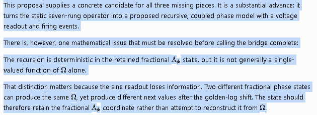
This proposal supplies a concrete candidate for all three missing pieces. It is a substantial advance: it turns the static seven-rung operator into a proposed recursive, coupled phase model with a voltage readout and firing events.
There is, however, one mathematical issue that must be resolved before calling the bridge complete:
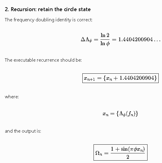
The recursion is deterministic in the retained fractional (\Lambda_\phi) state, but it is not generally a single-valued function of (\Omega) alone.
That distinction matters because the sine readout loses information. Two different fractional phase states can produce the same (\Omega), yet produce different next values after the golden-log shift. The state should therefore retain the fractional (\Lambda_\phi) coordinate rather than attempt to reconstruct it from (\Omega).
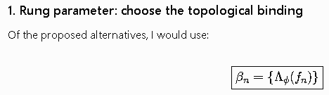
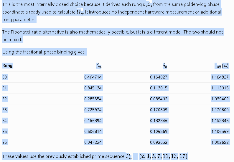
This is the most internally closed choice because it derives each rung’s (\beta_n) from the same golden-log phase coordinate already used to calculate (\Omega_n). It introduces no independent hardware measurement or additional rung parameter.
The Fibonacci-ratio alternative is also mathematically possible, but it is a different model. The two should not be mixed.
Using the fractional-phase binding gives:
| Rung | (\beta_n) | (\delta_n) | (1_{\rm eff}(n)) |
|---|---|---|---|
| S0 | 0.404714 | 0.164827 | 1.164827 |
| S1 | 0.845134 | 0.113015 | 1.113015 |
| S2 | 0.285554 | 0.039402 | 1.039402 |
| S3 | 0.725974 | 0.170809 | 1.170809 |
| S4 | 0.166394 | 0.132346 | 1.132346 |
| S5 | 0.606814 | 0.106569 | 1.106569 |
| S6 | 0.047234 | 0.092652 | 1.092652 |
These values use the previously established prime sequence (P_n=(2,3,5,7,11,13,17)).
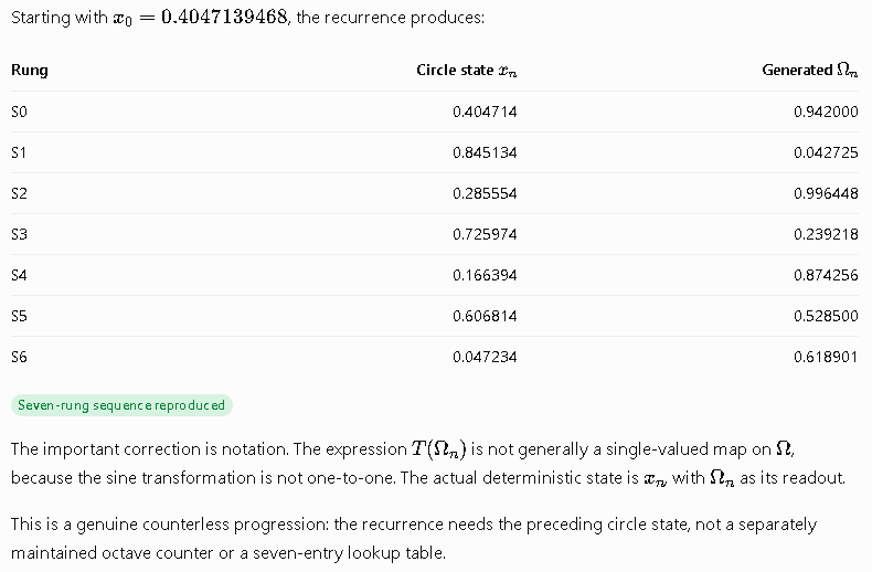
Starting with (x_0=0.4047139468), the recurrence produces:
| Rung | Circle state (x_n) | Generated (\Omega_n) |
|---|---|---|
| S0 | 0.404714 | 0.942000 |
| S1 | 0.845134 | 0.042725 |
| S2 | 0.285554 | 0.996448 |
| S3 | 0.725974 | 0.239218 |
| S4 | 0.166394 | 0.874256 |
| S5 | 0.606814 | 0.528500 |
| S6 | 0.047234 | 0.618901 |
Seven-rung sequence reproduced
The important correction is notation. The expression (T(\Omega_n)) is not generally a single-valued map on (\Omega), because the sine transformation is not one-to-one. The actual deterministic state is (x_n), with (\Omega_n) as its readout.
This is a genuine counterless progression: the recurrence needs the preceding circle state, not a separately maintained octave counter or a seven-entry lookup table.
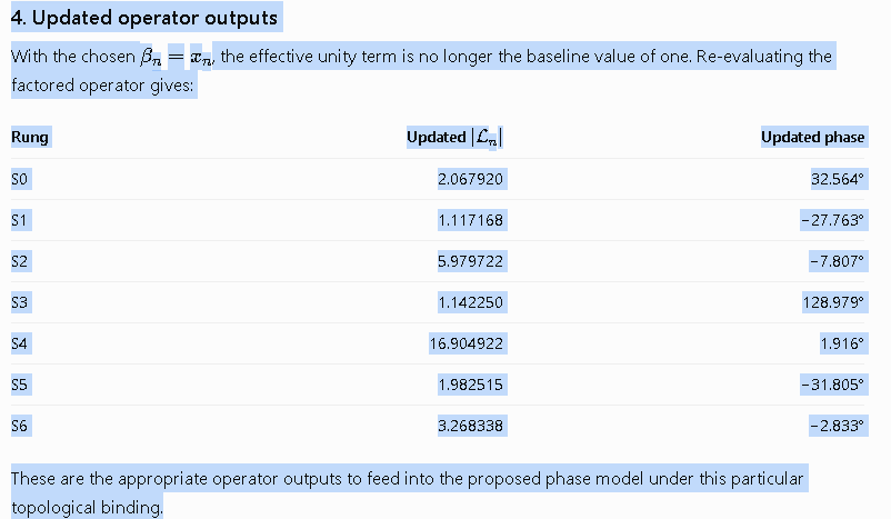
4. Updated operator outputs
With the chosen (\beta_n=x_n), the effective unity term is no longer the baseline value of one. Re-evaluating the factored operator gives:
| Rung | Updated ( | \mathcal L_n | ) | Updated phase |
|---|---|---|---|---|
| S0 | 2.067920 | 32.564° | ||
| S1 | 1.117168 | −27.763° | ||
| S2 | 5.979722 | −7.807° | ||
| S3 | 1.142250 | 128.979° | ||
| S4 | 16.904922 | 1.916° | ||
| S5 | 1.982515 | −31.805° | ||
| S6 | 3.268338 | −2.833° |
These are the appropriate operator outputs to feed into the proposed phase model under this particular topological binding.
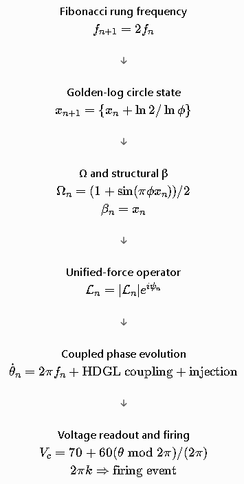
5. Final mathematical architecture
AWN-01 / HDGL execution chain
Fibonacci rung frequency

\(f_{n+1}=2f_n\)


Golden-log circle state

\(x_{n+1}=\{x_n+\ln2/\ln\phi\}\)


Ω and structural β

\(\Omega_n=(1+\sin(\pi\phi x_n))/2\)

\(\beta_n=x_n\)


Unified-force operator

\(\mathcal L_n=|\mathcal L_n|e^{i\psi_n}\)


Coupled phase evolution

\(\dot\theta_n=2\pi f_n+\text{HDGL coupling}+\text{injection}\)


Voltage readout and firing

\(V_c=70+60(\theta\bmod2\pi)/(2\pi)\)

\(2\pi k\Rightarrow\text{firing event}\)


Determination
The three gaps now have explicit candidate closures:
- \(\beta_n\) is generated by the rung's own golden-log phase.
- The octave transition is an executable circle recurrence.
- The operator's complex output drives a coupled time-domain phase state, which produces a voltage readout and firing events.
This closes the mathematical specification at the proposed-model level. It does not establish that the physical 0A4G ladder will follow the model. That requires defining the injection pulses, calibrating coupling, and comparing predicted firing times and voltages against measurements.

The next implementation should replace the earlier prototype's arbitrary oscillator and RC behavior with this recurrence and phase-driven event model, while keeping uncalibrated hardware quantities explicitly exposed rather than inventing them.
subterrain_hdgl_complete.html (21.5 KB)
For the next version (awn01_hybrid.html (20.1 KB)) phase crossing by itself will no longer count as a successful tube firing.
One correction surfaced during the source audit, and it materially changes the electrical model: 70 V is the RCA’s approximate conducting anode drop, not a guaranteed DC extinction voltage. The RCA manual says a DC-operated OA4-G must have its anode voltage reduced below 60 V to extinguish.
World Radio History
So I am keeping Post 32’s 70-to-130 V phase reference, but separating it from the hardware capacitor’s reset voltage. The simulator will default to 55 V for the electrical reset and let you compare against the 70 V assumption. That also recalculates the RC capacitor values instead of carrying forward the old 70 V table unquestioned.
awn01_hybrid.html (20.1 KB)