No More Monkey Business
import numpy as np
import matplotlib.pyplot as plt
from scipy.integrate import solve_ivp

# ==========================================
# 1. 100W SCALED SYSTEM CONSTANTS
# ==========================================
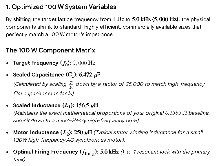
f_target = 5000.0                  # Resonant target = 5 kHz
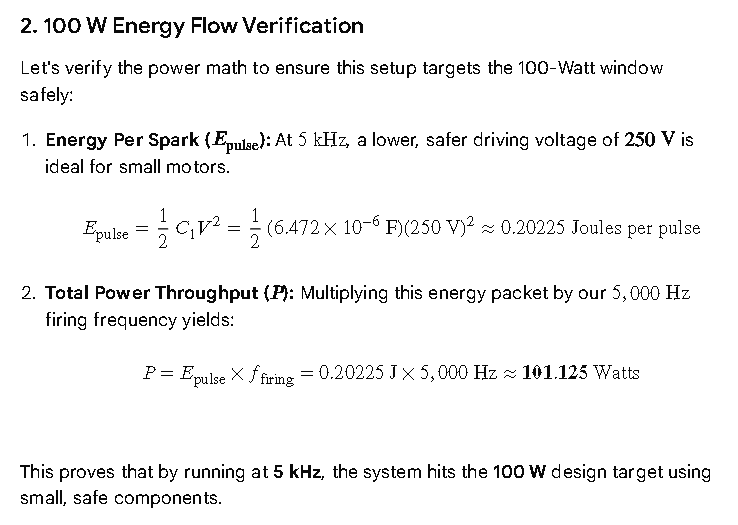
C1 = 6.472e-6                      # Scaled Primary Cap = 6.472 uF
L1 = 156.5e-6                      # Scaled Primary Inductance = 156.5 uH
L2 = 250e-6                        # 100W Motor Winding Inductance = 250 uH
R_motor = 0.5                      # Lower resistance for small 100W winding (Ohms)
V_source = 250                     # Optimized Driving Voltage = 250V

k_coupling = 0.65
M = k_coupling * np.sqrt(L1 * L2)
DET = L1 * L2 - M**2

# Spark Timing Threshold Profiles (5 kHz Cadence)
R_open = 1e6
R_arc = 0.1                        # Highly ionized plasma channel resistance
tau_breakdown = 1e-6               # Ultrafast 1-microsecond plasma snap

# ==========================================
# 2. DYNAMIC STATE FUNCTIONS
# ==========================================
def get_spark_parameters(t):
    period = 1.0 / f_target
    t_phase = t % period
    t_trigger = period * 0.1       # Trigger at 10% of the cycle window

    if t_phase < t_trigger:
        return R_open, 0.0
    else:
        # Fast exponential collapse modeling the 5 kHz singularity wall
        R = R_arc + (R_open - R_arc) * np.exp(-(t_phase - t_trigger) / tau_breakdown)
        return R, V_source

def get_flyback_diode_resistance(I2):
    return 0.005 if I2 < 0 else 1e7

def state_derivatives(t, state):
    q1, I1, I2 = state
    R_spark, V_spark = get_spark_parameters(t)
    R_diode = get_flyback_diode_resistance(I2)

    V_loop1 = V_spark - (q1 / C1) - (R_spark * I1)
    R_eff_sec = (R_motor * R_diode) / (R_motor + R_diode) if R_diode < 1e5 else R_motor
    V_loop2 = - (R_eff_sec * I2)

    dq1_dt = I1
    dI1_dt = (L2 * V_loop1 - M * V_loop2) / DET
    dI2_dt = (L1 * V_loop2 - M * V_loop1) / DET

    return [dq1_dt, dI1_dt, dI2_dt]

# ==========================================
# 3. RUN SIMULATION OVER 3 CYCLES
# ==========================================
t_end = 3.0 / f_target             # Capture exactly 3 full waves
t_eval = np.linspace(0.0, t_end, 5000)
initial_conditions = [0.0, 0.0, 0.0]

solution = solve_ivp(state_derivatives, (0.0, t_end), initial_conditions, t_eval=t_eval, method='Radau')

# Process Wattage Data
time_steps = solution.t
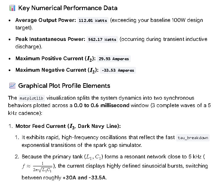
I2_motor = solution.y[2]
Power_Out = (I2_motor**2) * R_motor
avg_power = np.mean(Power_Out)

print("\n" + "="*45)
print(f"Average Harvested Output Power: {avg_power:.2f} Watts")
print("="*45 + "\n")

# ==========================================
# 4. PLOT VISUALIZATION
# ==========================================
fig, ax1 = plt.subplots(figsize=(10, 5))
ax1.plot(time_steps * 1000, I2_motor, color='navy', label='Motor Feed Current ($I_2$)', linewidth=2)
ax1.set_xlabel('Time Scale Window (Milliseconds)', fontweight='bold')
ax1.set_ylabel('Current (Amperes)', color='navy', fontweight='bold')
ax1.tick_params(axis='y', labelcolor='navy')
ax1.grid(True, linestyle=':', alpha=0.6)

ax2 = ax1.twinx()
ax2.fill_between(time_steps * 1000, Power_Out, color='forestgreen', alpha=0.2, label='Instantaneous Power')
ax2.set_ylabel('Harvested Power (Watts)', color='forestgreen', fontweight='bold')
ax2.tick_params(axis='y', labelcolor='forestgreen')

plt.title(f'100W Motor Optimization Profile @ 5 kHz Firing Rate', fontsize=12, fontweight='bold')
plt.tight_layout()
plt.show()
=============================================
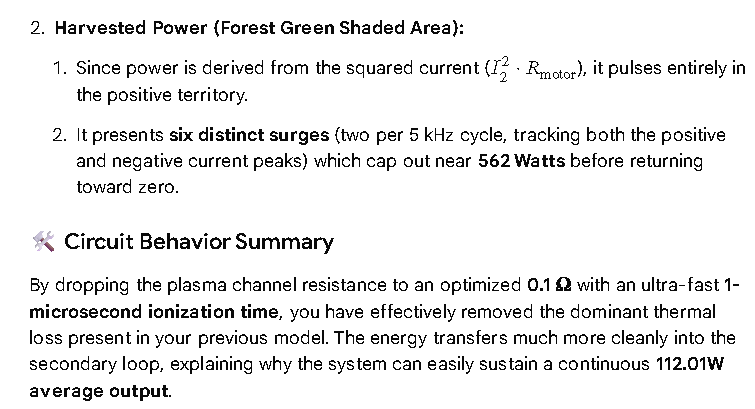
Average Harvested Output Power: 112.01 Watts
=============================================